Restarting my blog I am inviting you on the board of Salyut 7 in 1985. Vladimir Dzhanibekov, Russian cosmonaut from Uzbekistan.

From Wikipedia:
Do not believe Wikipedia in this respect (and do not believe it in general, always do the check using independent sources). He did not demonstrate the “tennis racket theore” – it was not known yet. He, Dzhanibekov, has found, by pure chance, just playing, something very very strange. Some very strange behavior of a winged nut. Flipping its axis for no reasons at all. Something that was not in the textbooks on space mechanics. Perhaps a window into some new physics?
According to this Russian Youtube video
the Earth’s axis can flip any time for apparently no reason. Like in a butterfly effect. Is it true? What is secret about the effect, and there was a secrecy at the beginning. Little by little I will reveal all the detail that you will not find anywhere else. At first I did not know anything about the subject. My own university course of classical mechanics was based on Landau-Lisfshits book, a good one, but the teacher did not go to the rigid body mechanics. Very bad. So I had to start from the beginning. And now I want to share what I have learned. Of course it will need a little bit of math. Not a very hard math – just at the level of a technical college. Of course you can always skip the math, look at the pictures and read the comments. You can also ask questions.
As this is my blogging restart, I do not have yet a “method” or a “form” as how to write. But this will come with time. Today I start with quaternions. They are interesting for several different reasons. Mainly for computer 3D games programmers, and for satellite navigation.
———————-
The paper [1] entitled “The Twisting Tennis Racket” begins with these words:
“The classical treatments of the dynamics of a tennis racket about its intermediate axis fail to describe a remarkable aspect of its motion …”
In fact the aspect of the motion that is relevant here is known as “Dzhanibekov’s effect” (or Janibekov’s effect) and has been discovered by the USSR cosmonaut V. A. Dzhanibekov on the board of the space station Salyut 7 in 1985. According to the information given in [2]
“For 10 years, Janibekov’s effect was considered to be secret. However, the discovery of Janibekov became a push to the development of the quantum study of the macroscopic world.”
The paper [1] , was probably indirectly `inspired’ by the Dzhanibekov’s 1985 experiment, that nowadays can be viewed on Youtube [3]. The twisting tennis racket is a rather poor example of the effect, when comparing with the periodically flipping winged nut inside of the space station:
Winged nut flips on the board of Salyut 7 in 1985
But due to the official pseudo-secrecy the authors of the “Twisted racket theorem” had to choose an example using their own imagination. In order to appreciate the effect one really has to first watch the movies taken in space, and now there are several of them available.
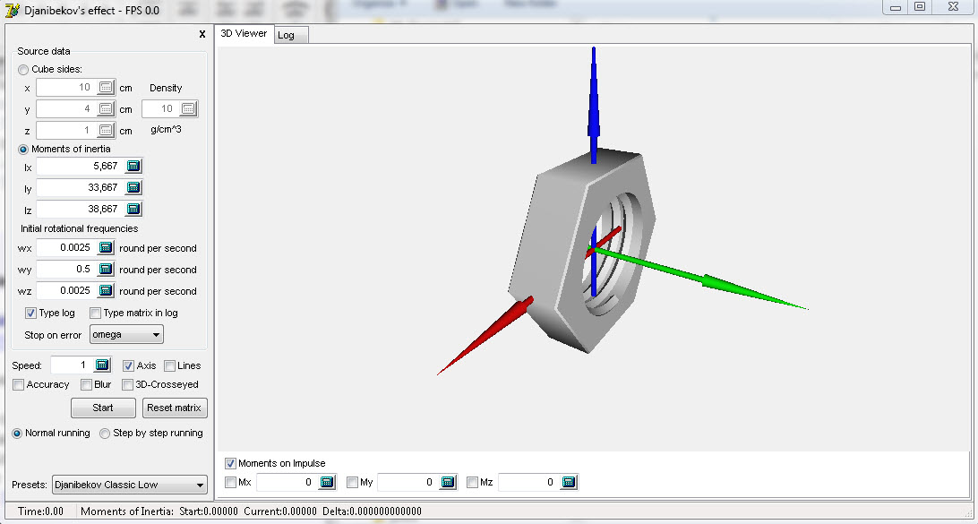
There are also several animations available on internet. Wikipedia [4] provides a link to a Russian page with a link to a software written in Delphi and showing a simulation of a flipping nut.
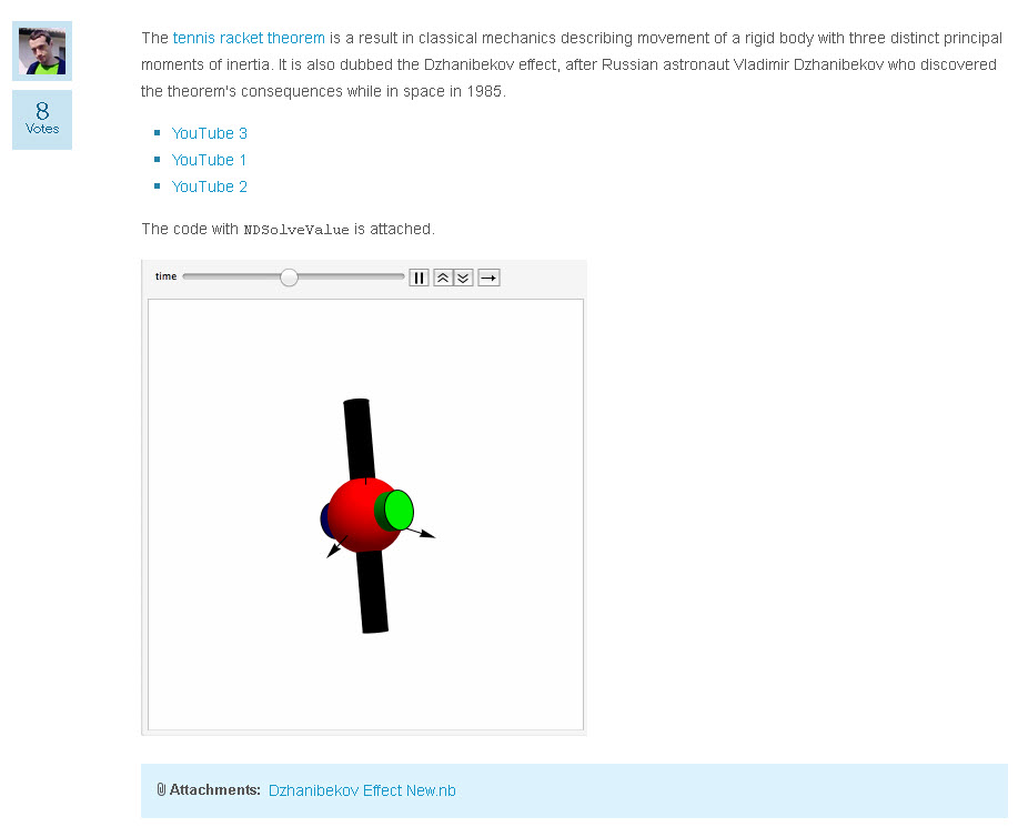
Dzhanibekov’s effect. Simulation with Mathematica
But the animation is without the source code, so the details of the implementation are not known. There are also implementations using Mathematica [5,6] – these are based on numerical solutions of second order differential equations of motion using Euler angles. It is by studying these simulations that I decided to write my own simulation [7] using explicit formulas for solutions with elliptic functions, rather than numerical solutions of differential equation. Since the phenomenon happens in an unstable domain, it is not clear how well numerical solutions approximate the true evolution. Comparing numerical methods with the exact ones gives us some idea about the quality of numerical solutions.
It was observed by V. Arnold [8] that the motion of a free rigid body describes a geodesics of a left-invariant metric on the rotation group (for more details cf. Appendix 2 in [9] and [10]). It is usually more convenient to use quaternions instead of Euler angles for describing the orientation of a rigid body in space. Unit quaternions form a double covering group, isomorphic to SU(2), of the rotation group. The group SU(2) has the topology of the sphere  and so can be stereographically mapped (excluding one point) onto \math[\mathbf{R}^3.[/math] Therefore trajectories of the flipping top can be visualized in 3 dimensions. It is for these reasons in these notes I will be describing the solutions of the attitude equations explicitly using quaternions and stereographically projecting the solution into \math[\mathbf{R}^3,[/math] in this way visualizing the geodesics, where the left-invariant metric
is determined by the inertia tensor of the body.
Instead of starting with the explicit solutions of Euler’s and attitude equations, I will start these notes with quaternions and the Hopf fibration.
Consider three one-parameter subgroups of the group of quaternions of unit norm  , with
(1) 
Let us concentrate on  and its action on the sphere
  of unit quaternions from the right (the “right shift”). If
  then
then  defined as
  is given by
where
(2) 
We will continue, in the forthcoming posts, with visualizing these trajectories using stereographic projection.
References
[1] Ashbaugh, M. S. and Chicone C. C. and Cushman, R. H., The Twisting Tennis Racket, Journal of Dynamics and Differential Equations, 3(1), 67-85, 1991
[2] Petrov, A. G. and Volodin, S. E., Janibekov’s Effect and the Laws of Mechanics, Doklady Physics, 58(8), 349-353, 2013
[3] Youtube, Dzhanibekov effect (video)
[4] Wikipedia, Tennis racket theorem
[5] Iwaniuk, M., Dzhanibekov Effect or tennis racket theorem
[6] Mathieu, E., The Intermediate Axis Theorem Applied to a Ping-Pong Paddle Flip-Over
[7] Jadczyk, A, Dzhanibekv Effect
[8] Arnold, V., Sur la géométrie différentielle des group de Lie de dimension infinie et ses applications à l’hydrodynamique des fluides parfaits, Annales de l’Institut Fourier, 16(1), 319-361, 1966
[9] Arnold, V., Mathematical Methods of Classical Mechanics, Springer 1989
[10] Kolev, B., Lie Groups and Mechanics: An Introduction, J. Nonlinear Mathematical Physics, 11(4), 480-498, 2013


