The recollections in the last post were incomplete. So, here is the continuation.
We have derived the property

On the other hand we stressed the fact that
 :
:
(2) 
is the rotation matrix that describes the rotation about the axis in the direction by an angle  .
.
From these two properties we can deduce the third one:
 is a rotation, then rotation about the vector
  by the angle
To deduce this last property we use the fact that for any  and any invertible
  we have:
![\[ e^{RXR^{-1}}=Re^XR^{-1}.\]](http://arkadiusz-jadczyk.eu/blog/wp-content/ql-cache/quicklatex.com-c22170d45c993125904651ab32f6ae0c_l3.png "Rendered by QuickLaTeX.com")
The proof of the above follows by expanding  as a power series, and noticing that
I will use spin equivalent of Eq. (3) when explaining how exactly I got the two images from the last post that I am showing again below:
The advantage in using Eq. (3) is that it may be easy to calculate the exponential  but not so easy the exponential
Our aim is to draw trajectories in the rotation group  made by the asymmetric top spinning about its largest moment of inertia axis, which in our setting is the third axis. As the rotation group is not very graphics friendly, we are using the double covering group
  or, equivalently, the group of unit quaternions. We then use stereographic projection to project trajectories from the 3-dimensional sphere
  to 3-dimensional Euclidean space
But first things first. Before doing anything more we first have to translate the above properties into the language of  Therefore another recollection is necessary at this point. In Pauli, rotations and quaternions we have defined three spin matrices:
(4) 
In Putting a spin on mistakes we have explained that we have the map  that associates rotation matrix
  to every matrix
  in such a way that for every vector
  we have
(5) 
It follows immediately from the above formula that is a group homomorphism, that is we have
(6) 
At the end of Putting a spin on mistakes we have arrived at the formula:
(7) 
which tells us that the matrix  defined as
(8) 
describes the rotation about the direction of the unit vector  by the angle at the level.
The map is 2:1. We have  Matrices
  and
and  implement the same rotation. When changes from
  to
to  the matrix in Eq. (7) describes the full
  turn, but the matrix becomes
  rather than
  . We need to make
  rotation at the
  vector level to have rotation at the spin level. That is described by
  in the exponential in Eq. (7).
At the spin level we then obtain the following analogue of Eq. (\ref:rqr}):

Now we can finally look back at the images of trajectories. In Seeing spin like an artist we noticed that rotation about the z-axis is described by the matrix
(10) 
while rotation by the angle  about y-axis is described by the matrix
(11) 
 describes uniform rotation of the top about its z-axis, when the z-axis of the top and of the laboratory frame are aligned. As observed in Towards the road less traveled with spin that is not an interested path for drawing. To make the path more interesting we tilt the laboratory frame. To this end we use, for instance, the matrix
  with
with 
(12) 
Now the axis of rotation of the top is tilted by 30 degrees with respect to the z-axis of the laboratory frame. We get new path of the evolution in the group
(13) 
From Eq. (1) in Chiromancy in the rotation group we can now calculate real parameters  For a general matrix the formulas are:
(14) 
In our particular case we get:
(15) 
We then get rather awfully looking the parametric formulas for the stereographic projection:
(16) 
The result (running  from to
  ) is not very interesting – just a circle:
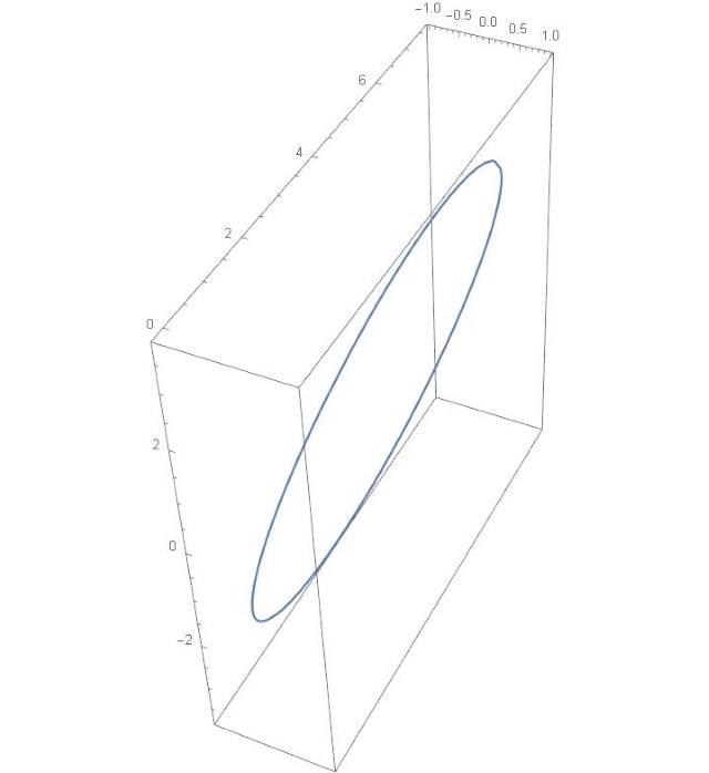
It is better than the straight line with a non tilted top, but not a big deal. But the next thing we want to do is to rotate the tilt axis in the (x,y) plane, that is about the  -axis of the laboratory. If we want to rotate by an angle
  we should replace by
  – according to Eq. (9). That is we should look at the trajectory:
![\[U'(t,\psi)=U(\psi)V(\phi)U^*(\psi)U(t).\]](http://arkadiusz-jadczyk.eu/blog/wp-content/ql-cache/quicklatex.com-7777f3a43a8a37e890e2aa58366362c7_l3.png "Rendered by QuickLaTeX.com")
Now,  Since anyway we are are going to run with through the whole
  interval, we can as well use instead of
  Therefore we can draw
![\[U'(t,\psi)=U(\psi)V(\phi)U(t).\]](http://arkadiusz-jadczyk.eu/blog/wp-content/ql-cache/quicklatex.com-7ab684324f55a588bb0a6d6b896cc75f_l3.png "Rendered by QuickLaTeX.com")
We can calculate  and then
  Here are the results from my Mathematica code:
(17) 
(18) 
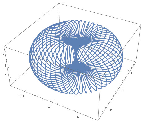
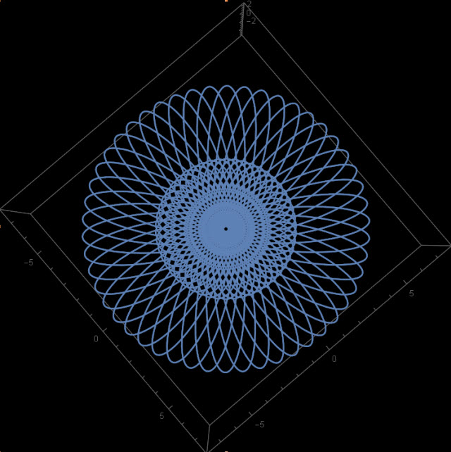
And here is the resulting of plotting 30 such circles, each for  with
with  increasing from 0 t0 180 degrees, every 6 degrees:
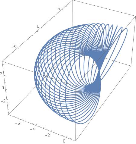
It looks like half of a torus. With  we get another, larger torus …
In the next posts we will disturb the motion of the top to see what kind of trajectories we will be getting then.


