In this note I will repeat some stuff that I was already explaining in the past, but we will also find some important new stuff.
The time evolution differential equation for the attitude matrix  is
is
(1) 
where  is the angular velocity vector in the body frame, and
  maps any vector
  into skew-symmetric matrix as follows:
(2) 
It has the property that for any vector  we have
(3) 
Equation (1) follows immediately from the definition of the angular velocity. The angular velocity  in the laboratory frame is defined by
(4) 
But  maps coordinates of vectors in the body frame into their coordinates in the laboratory frame. Thus
  and therefore
(5) 
But from Eq. (3) we have  therefore
![\[QW(\boldsymbol{\Omega}) Q^*=\dot{Q}Q^*,\]](http://arkadiusz-jadczyk.eu/blog/wp-content/ql-cache/quicklatex.com-2b8dc2bd14afb26bb4a8b5bbc51a531a_l3.png "Rendered by QuickLaTeX.com")
and so Eq. (1) follows.
While description of rotations in terms of orthogonal  matrices in principle suffices in classical mechanics, sometimes it is convenient to use the group of quaternions of unit norm, the group isomorphic to the group
  used in quantum mechanical description of half-integer spin particles. Quaternions have some advantages in numerical procedures (as for instance in 3D computer games), but they are also convenient for graphical representation of the intrinsic geometry of the rotation group. And this is what interests us, when we plot trajectories representing history of a spinning rigid body.
Quaternions of unit norm, representing rotations, form a 3-dimensional sphere in 4-dimensional Euclidean space, and we are projecting stereographically this sphere onto our familiar three-dimensional space, where we orient ourselves in a usual way known from everyday experience.
The question therefore arises: how the equation describing the time evolution looks like when represented in the quaternion setting?
To derive it we have to return to the fundamental relation between quaternions and rotations of vectors in space.
For every vector  with components
  denote by
  the pure imaginary quaternion defined as:
(6) 
Then to unit quaternion  that is such that
  there corresponds rotation matrix
  such that for all the following identity holds
(7) 
The second interesting property of the hat map is that for all  we have
(8) ![\begin{equation*}[\hat{\mathbf{v}},\hat{\mathbf{w}}]=2\widehat{\mathbf{v}\times\mathbf{w}},\end{equation*}](http://arkadiusz-jadczyk.eu/blog/wp-content/ql-cache/quicklatex.com-9d54d4425ed3ea3d47077fe970c7b63d_l3.png "Rendered by QuickLaTeX.com")
where ![[\cdot,\cdot]](http://arkadiusz-jadczyk.eu/blog/wp-content/ql-cache/quicklatex.com-641143f73744dffa48c2e2846c7cda21_l3.png "Rendered by QuickLaTeX.com") is the commutator. The property follows directly form the definitions and from the quaternion multiplication rules. Every pure imaginary quaternion is of the form for some
is the commutator. The property follows directly form the definitions and from the quaternion multiplication rules. Every pure imaginary quaternion is of the form for some 
As shown on plaque by the Royal Canal at Broome Bridge in Dublin,
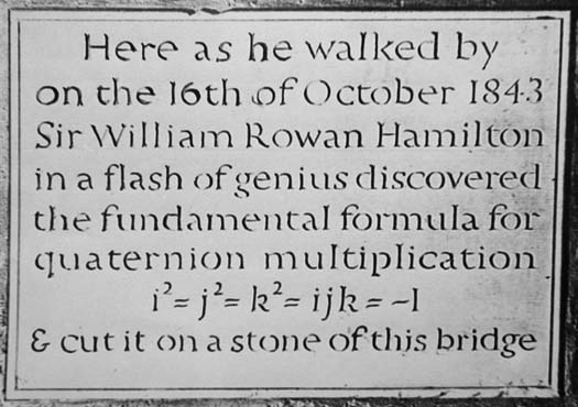
the essence of the quaternions is contained in the four equations
(9) 
From these, multiplying from the left and/or from the right by  or
or  or
or  we derive
(10) 
From the definition of the hat map we have
(11) 
Therefore
![\[ [\hat{\mathbf{v}},\hat{\mathbf{w}}]=\hat{\mathbf{v}}\hat{\mathbf{w}}-\hat{\mathbf{w}},\hat{\mathbf{v}}\]](http://arkadiusz-jadczyk.eu/blog/wp-content/ql-cache/quicklatex.com-725b7cd428fec4ef408d51c243ba72ed_l3.png "Rendered by QuickLaTeX.com")
![\[=(v_1\mathbf{i}+v_2\mathbf{j}+v_3\mathbf{k})(w_1\mathbf{i}+w_2\mathbf{j}+w_3\mathbf{k})-(w_1\mathbf{i}+w_2\mathbf{j}+w_3\mathbf{k})(v_1\mathbf{i}+v_2\mathbf{j}+v_3\mathbf{k}).\]](http://arkadiusz-jadczyk.eu/blog/wp-content/ql-cache/quicklatex.com-b9bd2f235f9a33de350dbd83e6bb88b5_l3.png "Rendered by QuickLaTeX.com")
When we expand the parenthesis and use the multiplication rules in Eqs. (9),(10), we find that the terms with squares cancel out, while the terms with products like  etc. can be organized as follows
![\[ [\hat{\mathbf{v}},\hat{\mathbf{w}}]=2\left[(v_2w_3-w_2v_3)\mathbf{i}+(v_3w_1-w_3v_1)\mathbf{j}+(v_1w_2-w_2v_1)\mathbf{k}\right].\]](http://arkadiusz-jadczyk.eu/blog/wp-content/ql-cache/quicklatex.com-5e713d35bb274918a7793c39b664351c_l3.png "Rendered by QuickLaTeX.com")
The coefficients in the parentheses on the right are now exactly the components of the cross product 
Thus
![\[[\hat{\mathbf{v}},\hat{\mathbf{w}}]=2\widehat{\mathbf{v}\times\mathbf{w}}.\]](http://arkadiusz-jadczyk.eu/blog/wp-content/ql-cache/quicklatex.com-4eccabc3e5b661a48d322e6e9cd33b4b_l3.png "Rendered by QuickLaTeX.com")
Suppose now that  is a trajectory in the space of unit quaternions, while is the corresponding trajectory in the rotation group. Thus we have
(12) 
for all  and all We now differentiate both sides with respect to
  On the left we use the standard product rule for differentiation, but we pay attention so as to preserve the order, because multiplication of quaternions is non commutative. On the right we enter with the differentiation under the “hat”, because it is a linear operation. We obtain:
(13) 
Assume now that is a solution of Eq. (1), so that  We have
(14) 
We now use Eq. (12) on the right to obtain
(15) 
In order to get rid of  we differentiate the defining equation of unit quaternions
  to obtain
(16) 
or
(17) 
Putting this into Eq. (15) and multiplying both sides on the right by  we obtain
(18) 
Multiplying from the left by  :
:
(19) 
From Eq. (16) it follows that the quaternion  is pure imaginary:
  Therefore there exists vector
  such that
(20) 
Eq. (19) can now be written as
(21) ![\begin{equation*}[\hat{\mathbf{w}},\hat{\mathbf{v}}]=\widehat{\boldsymbol{\Omega}\times\mathbf{v}},\end{equation*}](http://arkadiusz-jadczyk.eu/blog/wp-content/ql-cache/quicklatex.com-16c6976ac288aab8a167a93a1de765a6_l3.png "Rendered by QuickLaTeX.com")
where on the right we have used Eq. (3). Applying Eq. (8) to the left we end with
(22) 
Since the above holds for any we deduce that
(23) 
Using (20) we finally obtain:
(24) 
Note: It may be that the final formula can be derived in a shorter way, but I do not know how. It is this last formula that I was using when verifying that the algorithm provided in Meeting with remarkable circles gives indeed a solution of the evolution equation.


