I noticed that somehow I did not finish with the case  So today, without further ado, I am posting the algorithm.
We have the body with  and we are considering the case with
  , where
  is, as always, the ratio of the doubled kinetic energy to angular momentum squared.
Then we define
(1) 
(2) 
(3) 
(4) 
(5) 
(6) 
(7) 
(8) 
(9) 
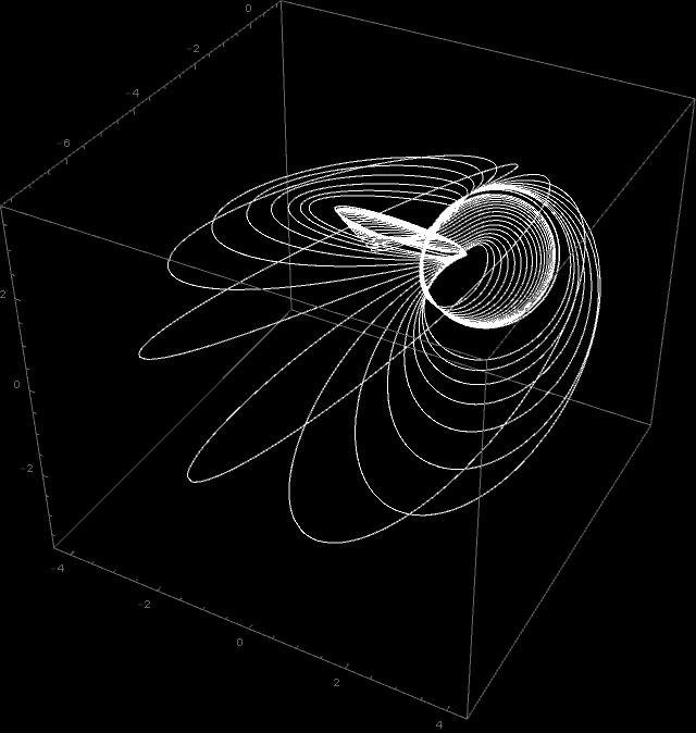
I use the above formulas to draw a stereographic projection of one particular path. So, I take  , and do the parametric plot of the curve
  in
in 
with
![\[\mathbf{r}(t)=\left(\frac{q_1(t)}{1-q_0(t)},\frac{q_2(t)}{1-q_0(t)},\frac{q_3(t)}{1-q_0(t)}\right).\]](http://arkadiusz-jadczyk.eu/blog/wp-content/ql-cache/quicklatex.com-9e9586446344017cc3859d919f8f5e33_l3.png "Rendered by QuickLaTeX.com")
I show below two plots. One with  and one with
  For this selected value of
  the time between consecutive flips, given by the formula
(10) 
So, for  we have somewhat less than 200 flips, and the lines are getting rather densely packed in certain regions.
Notice that is just one geodesic line, geometrically speaking the straightest possible line in the geometry determined by the inertial properties of the body.
It is this “geometry”that will become the main subject of the future notes.

How can such a line be “straight”? Well, it is….


