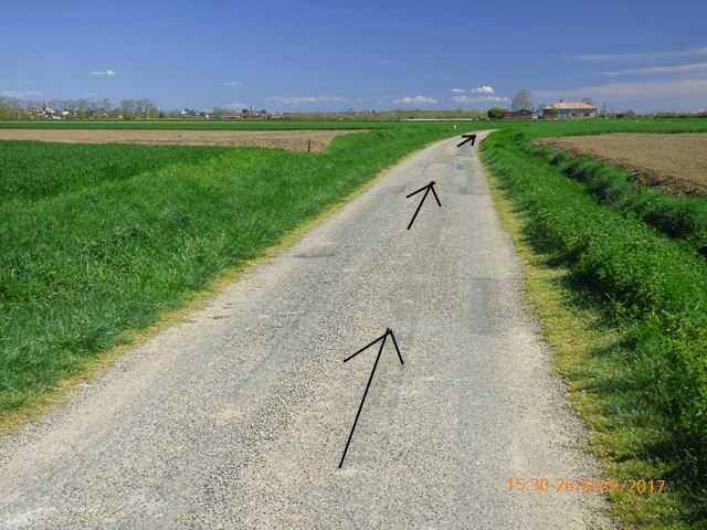
Whenever there is a path, there are vectors tangent to that path. Like here, on the picture below. I went outside for a walk, in search of vector fields. At first couldn’t find any, but then I realized that there is a vector tangent to my path, at every point of my path. Here are three such vectors:
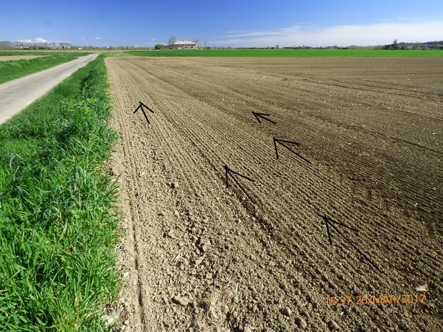
But then, I looked to the right of the path, and there I saw a real, two-dimensional field of vectors.
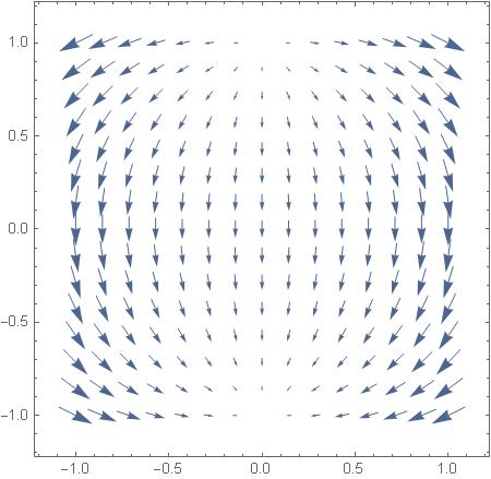
Then, at home, I used Mathematica to produce an artificial vector field:
And I have generated its stream lines:
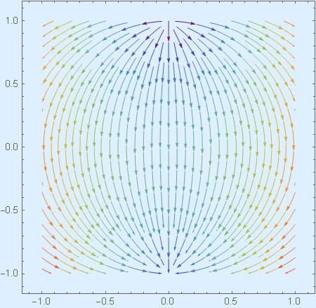
To every vector field we have associated flow represented by steam lines, and to every flow of stream lines we have associated vector field. We generate stream lines from vector field by integration, we generate vector filed from flow of stream lines through differentiation.
Here is how I did it in order to create the two graphs above:
I thought about one-parameter family of transformations on the complex plane, but not too trivial one. Something that I did not know in advance how exactly it would look like. The following has occurred to me:
![\[f_t:z\mapsto \frac{\cosh(t)z-i\sinh(t)}{i\sinh(t) z+\cosh(t)},\]](http://arkadiusz-jadczyk.eu/blog/wp-content/ql-cache/quicklatex.com-45c044df9ee4f23ba815416a3f91af08_l3.png "Rendered by QuickLaTeX.com")
where  Notice that
  and
and  To check the first property takes a little bit of calculations. In order to obtain the vector field from this “flow of complex numbers” I am calculating the derivative:
![\[X(z)=\frac{d}{dt} f_t(z)|_{t=0}.\]](http://arkadiusz-jadczyk.eu/blog/wp-content/ql-cache/quicklatex.com-bafc4f7e930926a2394a4b227ec731a5_l3.png "Rendered by QuickLaTeX.com")
I used Mathematica to get
![\[X[z]=-i(1+z^2).\]](http://arkadiusz-jadczyk.eu/blog/wp-content/ql-cache/quicklatex.com-b69f5ebd7d9188ca293aaeb5773f0a10_l3.png "Rendered by QuickLaTeX.com")
To draw this vector field on the  plane I write
  and calculate
![\[-i(1+(x+iy)^2)=-i(1+x^2-y^2+2ixy)=2xy+i(-1+y^2-x^2)\]](http://arkadiusz-jadczyk.eu/blog/wp-content/ql-cache/quicklatex.com-381d42e462ddef3269aeb8747edb128e_l3.png "Rendered by QuickLaTeX.com")
So
![\[ X(x,y)= (\mathrm{Re} (X(z)),\mathrm{Im}(X(z))=(2xy,y^2-x^2-1).\]](http://arkadiusz-jadczyk.eu/blog/wp-content/ql-cache/quicklatex.com-be321c0f4c534b6b896c8b1801ac25ac_l3.png "Rendered by QuickLaTeX.com")


I want outside ->
I went outside
looked to the left ->
looked to the right
graphs about ->
graphs above
?
?
therefore my ->
Therefore my
the re ->
there
With in
in  , there is no real problem for
  . ->
. ->
?
First I tried to fix the original example, but after a while decided to give an example that will be useful in the future. Thanks for noticing my erroneous attempt immediately.
Yes, Bjab, lot of errors. Not just “mistakes”. Serious errors. Will have to rewrite it all. Probably replacing z^t with z^(e^t). But then the vector field will be more interesting – which is good.
Edit: It will not work. For complex numbers (z^x)^y is, in general not the same as z^(xy). So, I can produce vector fields this way, but I will not know what is their meaning. What I need is a a good sleep. Perhaps the Goddess of Ramanujan will give me advice. I was watchin the movie about him two days ago. But I also have the book. The movie does not tell the truth!
Ark,
did you mean hyperbolic sine in numerator?
I think you meant it.
But then derivative is slightly different.
I calculated it as:
In fact, there were two mistakes. First it was sinh, indeed, but then, there was also the sign. I corrected both. Thanks!
Oh, when there is minus in numerator even I can check that holds.
So there should be “-1” in equation before last.
Yes. Missed in action. Restored now. Thanks.
I am not sure how to plot the streamlines. Ploted the vector field ok. I then integrated both terms of X(x,y)wrt time to get and
and  .
.
It produced the same shapes as your plots. Is that correct?
That is not correct. x and y on the trajectory (stream line) are functions of t. So, in Maple you solve differential equations:
sys_ode := (D(x))(t) = 2*x(t)*y(t), (D(y))(t) = y(t)^2-x(t)^2-1
You can set initial conditions:
ics := x(0) = x0, y(0) = y0
Then you solve:
dsolve([sys_ode, ics])
The solution looks complicated, but that is because it is written in terms of real and imaginary part of f_t from the post.
Now, having the solution with integration constants, you can plot streamlines as trajectories, as in
http://fr.maplesoft.com/applications/view.aspx?SID=6665&view=html
Thank You. Took me a while to figure it out but got there,
http://imgur.com/koUBrNY