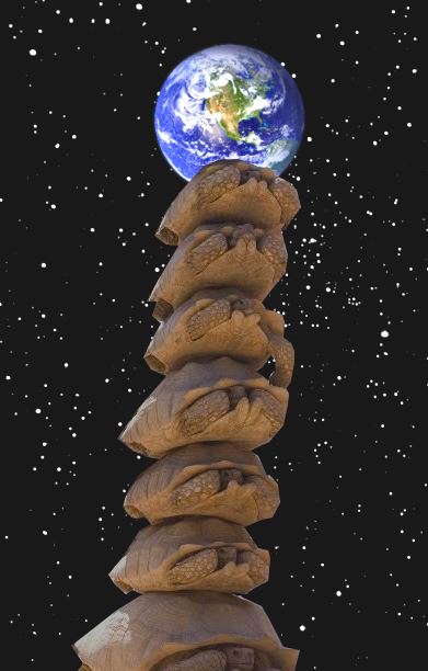
“Turtles all the way down” is an expression of the infinite regress problem in cosmology posed by the “unmoved mover” paradox. The metaphor in the anecdote represents a popular notion of the model that Earth is actually flat and is supported on the back of a World Turtle, which itself is propped up by a column of turtles.[1] Questioning what the final turtle might be standing on, the anecdote humorously concludes that it is “turtles all the way down”
The above quote comes from the Wikipedia entry Turtles all the way down
It is illustrated by the following story
After a lecture on cosmology and the structure of the solar system, William James was accosted by a little old lady.
“Your theory that the sun is the centre of the solar system, and the earth is a ball which rotates around it has a very convincing ring to it, Mr. James, but it’s wrong. I’ve got a better theory,” said the little old lady.
“And what is that, madam?” Inquired James politely.
“That we live on a crust of earth which is on the back of a giant turtle,”
Not wishing to demolish this absurd little theory by bringing to bear the masses of scientific evidence he had at his command, James decided to gently dissuade his opponent by making her see some of the inadequacies of her position.
“If your theory is correct, madam,” he asked, “what does this turtle stand on?”
“You’re a very clever man, Mr. James, and that’s a very good question,” replied the little old lady, “but I have an answer to it. And it is this: The first turtle stands on the back of a second, far larger, turtle, who stands directly under him.”
“But what does this second turtle stand on?” persisted James patiently.
To this the little old lady crowed triumphantly. “It’s no use, Mr. James – it’s turtles all the way down.”
—J. R. Ross, Constraints on Variables in Syntax 1967
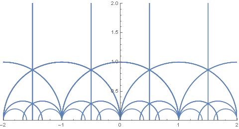
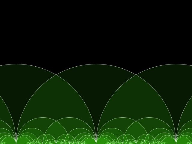
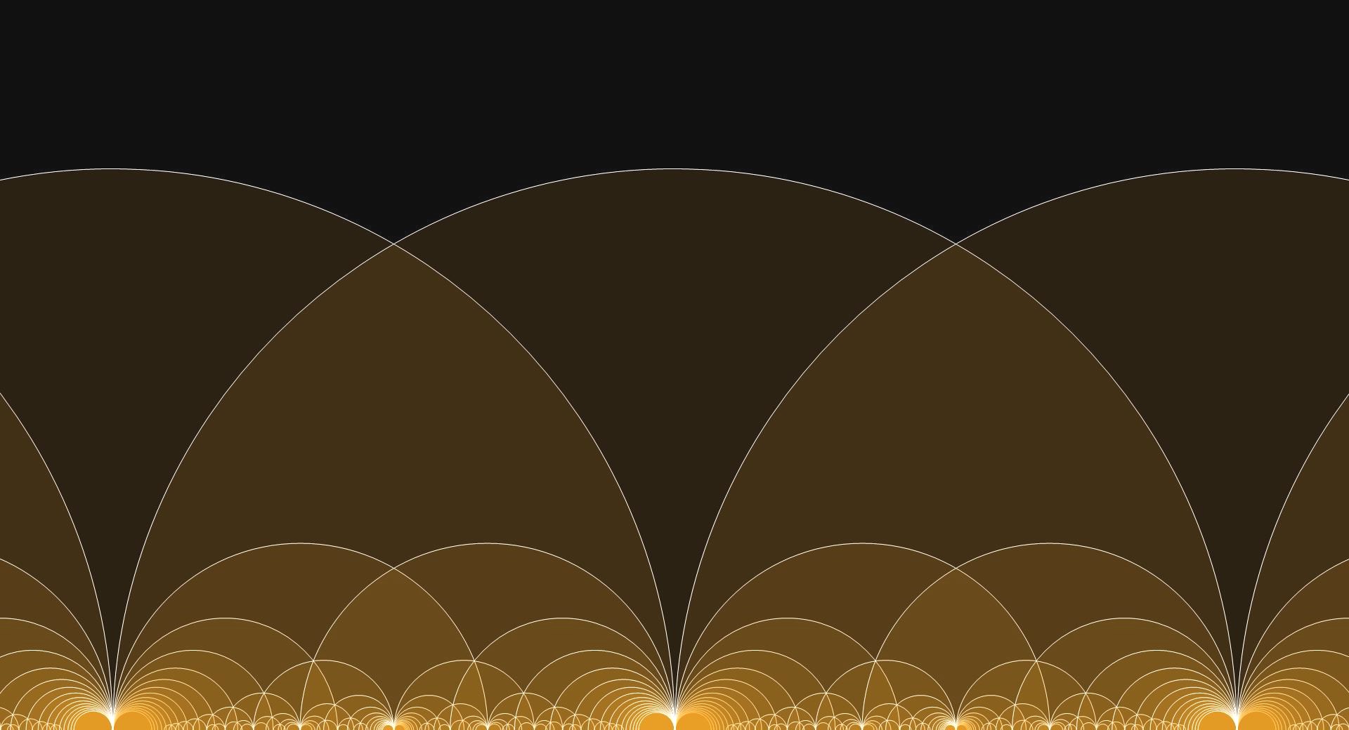
The Dedekind tessellation is a mathematical version of the flat Earth and turtles all the way down. Instead of the flat Earth we have the Poincaré disk, and instead of turtles we have circles – all the way down.
It is beautifully shown in the graphics taken from web pages of prof. J. Kocik from Department of Mathematics Southern Illinois University at Carbondale.

I have mentioned this subject at the end of Geodesics on the upper half-plane – parametrization, two days ago. In the meantime prof. Kocik was kind enough to send me his unpublished paper “A note on the Dedekind tessellation“. Looking inside I have found that I have made a mistake in my Mathematica program that was supposed to create my own version of the tessellation. After fixing my mistake (I have forgotten one term in my formula for the centers of the circles) I was able to create my own poor man version of the Dedekind tessellation (Kocik gives a simple method of computing the centers and the radii of all circles in the Dedekind tessellation!), and here I am going to explain, in details, how I did it.
Here is my final result that is a poor imitation of the beautiful and clever Kocik’s interactive graphics:
Instead of the disk it is better to use the upper half-plane, where the group SL(2,R) acts by fractional linear transformations. Let me recall the action. With
(1) 
the action on the upper half-plane, the set of complex numbers  with
with  is given by
(2) 
 defined as
  There is a simple relation between the two actions: we can obtain one action from another by composing it with the similarity transformation
 ![A\mapsto \left[\begin{smallmatrix}0&1\\1&0\end{smallmatrix}\right]A\left[\begin{smallmatrix}0&1\\1&0\end{smallmatrix}\right].](http://arkadiusz-jadczyk.eu/blog/wp-content/ql-cache/quicklatex.com-bbc039c143a5f3794ef8034ae02d10f7_l3.png "Rendered by QuickLaTeX.com")
The group SL(2,R) has a discrete subgroup SL(2,Z), often called the modular group, the group of  matrices with entries that are integers. For instance the following two matrices:
(3) 
In his online notes on SL(2,Z) Keith Conrad ( I recommend watching the great illusion on one of his web pages) shows that these two matrices generate (by taking inverses and products) the whole group SL(2,Z). In fact his  is transposed to the one above, but that does not matter.
Dedekind tessellation of the upper half-plane is an analogue of the tessellation of the usual Euclidean plane into squares of unit side length. All the plane can be nicely covered by translations of just one square, namely by translations by an integer amount in horizontal and vertical direction. In the case of the upper half-plane instead of a square we have a triangle, so called fundamental domain. In the picture below, taken from Condrad’s  paper, we see the (grayed) standard fundamental domain consisting of complex numbers with
  and
and 
Sure it does not look like a triangle, but it is a triangle, with the top vertex at infinity! The bottom side is a part of the unit circle – therefore a geodesic in the hyperbolic geometry we are dealing with.
By acting on this one triangle with matrices from the group SL(2,Z) we can nicely triangulate the whole upper half-plane – that is called the Dedekind tessellation. In Wikipedia article on Modular Group, in the section on Tessellation of the hyperbolic plane, it is accompanied with the following image:

Looking at this image it occurred to me that instead of acting on the fundamental domain I can as well act on the unit half-circle and on the two vertical lines. In order to do this I need a formula how elements of SL(2,Z) transform the unit circle and the two vertical lines. And I am interested in the resulting circles, I do not care about vertical lines as they do not add much to the tessellation. Using mathematical software (I use Mathematica most of the time) the task was not too difficult.
Suppose we have a circle of radius  with center at
  on the real axis. We apply the transformation
  to this circle using matrix
  in SL(2,R). The result is, as it can be verified without much difficulty using any computer algebra software, the circle
  with
with
(4) 
(5) 
We are interested in transformations of one particular circle with  and
and  Then the formulas simplify:
(6) 
(7) 
Of course we are interested only in the cases where the denominator is non zero.
Now suppose we have a vertical line at . It is transformed into a circle with
(8) 
(9) 
We are interested in two cases  and only when the denominator is non zero.
Using generators  above, taking their inverses and products, in different orders, I generated 35416 SL(2,Z) matrices. They can be downloaded as the file sl2.zip. The file has the format:

…
Separate matrices look as  .
.
I will describe now, step by step, how i have created Fig. 1 above, using Mathematica. It is certainly not an optimal way, but my description may help to understand how to create Dedekind tessellation using different methods.
m=Import[“H:/sl2z.m”];
x1[a_]:=(a[[1]][[2]]*a[[2]][[2]]-a[[1]][[1]]*a[[2]][[1]])/(a[[1]][[2]]^2-a[[1]][[1]]^2);
r1[a_]:=1/Abs[(a[[1]][[2]]^2-a[[1]][[1]]^2)];
r1i[a_]:=Abs[(a[[1]][[2]]^2-a[[1]][[1]]^2)];
These are the definitions of  as in Eqs. (6,7). The last one is the inverse of the radius. We want it to be
  Thus we create a sublist m1:
m1=Select[m, r1i[#]>0 &]
Then m1 has 35350 elements. We now use the first two lines to create the list of centers and radii:
mc = Table[{x1[m1[[i]]], r1[m1[[i]]]}, {i, 1, Length[m1]}];
But now there will be repeated elements in the list. To get rid of them I use
mc = Union[mc];
And I care only about circles with radius, say,  :
:
mc100 = Select[mc, #[[2]] > 1/100 &];
There are only 1923 such circles.
We can already do the plot:
The rest is optional. I added to these circles 12 circles obtained from the two vertical lines. Then I used paintnet software to invert the colors. The end result is in the Fig. 1 above.

![A=\left[\begin{smallmatrix}\lambda&\mu\\ \bar{\mu}&\bar{\lambda}\end{smallmatrix}\right]](http://arkadiusz-jadczyk.eu/blog/wp-content/ql-cache/quicklatex.com-2e511c5cae985c3970df6ef6d1883bab_l3.png "Rendered by QuickLaTeX.com") is a complex matrix from SU(1,1) with
is a complex matrix from SU(1,1) with  split into real and imaginary parts, then the real
  matrix
  from SO(2,1) is given by the formula:
 is a group homomorphism, that is
  and
and  ( Of course in
  identity matrices of different sizes.)

![A'=\left[\begin{smallmatrix}\alpha&\beta\\ \gamma&\delta\end{smallmatrix}\right]](http://arkadiusz-jadczyk.eu/blog/wp-content/ql-cache/quicklatex.com-8969b960a5764336f49fd61d00bb538d_l3.png "Rendered by QuickLaTeX.com") is a real matrix from SL(2,R) (i.e.
is a real matrix from SL(2,R) (i.e.  ), then
  is in SU(1,1). If we calculate explicitly
  and
and  in terms of
  the result is:


 , for instance in
 and
and  defined as
 is in sl(2,R), that is if
  is also of zero trace (we do not need the property of determinant one for this). The map
  is a linear map. Thus we have action, let us call it
  , of SL(2,R) on sl(2,R):
![\[\mathcal{L}(A_1A_2)=\mathcal{L}(A_1)\mathcal{L}(A_2).\]](http://arkadiusz-jadczyk.eu/blog/wp-content/ql-cache/quicklatex.com-eaf44c72fe09ddc3fb2e0378a0344943_l3.png "Rendered by QuickLaTeX.com")
 one writes
  and uses the term “adjoint representation”. In short: the group acts on its Lie algebra by similarity transformations. Similarity transformation of a generator is another generators. Even more, by expanding exponential into power series we can easily find that
 as follows
 is the trace of the product of matrices

 It is easy to calculate scalar products of the basis vectors. We get the following matrix for the matrix
  with entries

 has “time direction”, while
  are “space directions”.
 for
for ![A=\left[\begin{smallmatrix}\alpha&\beta\\ \gamma&\delta\end{smallmatrix}\right]](http://arkadiusz-jadczyk.eu/blog/wp-content/ql-cache/quicklatex.com-969779c63def79263f77beb857467082_l3.png "Rendered by QuickLaTeX.com") . Here is the result:
. Here is the result:
 is a vertical line, then
  therefore
  In
In 


 and
and  on the vertical line must be proportional:
 is an “affine parameter”: it is proportional to the arc length, possibly translated. In fact that is part of the definition of the geodesic that enters the “Noether’s theorem” that we are using. Usually we choose the proportionality constant equal to one.
 Choosing the constant equal to 1, we have

 is of unit length. In our case that is equivalent to
 or
or  or
or  , so that there are three kinds of geodesics. In physics this happens for space-time metrics with Minkowski signature, and in multi-dimensional Kaluza-Klein theories. We will discuss another such case in the following posts.
 is some function of the arc length parameter
  , and substitute into Eqs. (