In the recent note “SL(2,R) generators and vector fields on the half-plane” we got acquainted with two particular simple symmetries of the non-Euclidean hyperbolic geometry of the complex upper half-plane  These two symmetries are horizontal translation and uniform dilation. The horizontal translational symmetry means that all geometric properties of objects are invariant when all parts of the object keep the same height (constant
  ), and only the
  coordinate is translated by a fixed amount. The symmetry with respect dilations means that when we multiply all coordinates by a certain positive number, then we should also multiply the coordinates by the same number. We obtain this way not only an object that is similar to the original, but, moreover, it also has the same size!
In Hyperbolic angels and demonswe were playing with “equal sizes” of Esher’s angels and demons on the Poincare disk:

Today we will use the Cayley transform and move the Esher’s art piece to the upper half-plane.

The exact name of the image we will be playing with is Circle Limit IV. We want to render this image on the upper half-plane using Cayley transform. The problem that we need to address is this: to render the whole circle, we would need the whole upper half-plane. But we can only show a finite part of the plane. Therefore we need to decide how to cut?
I created a little Mathematica program to help me with this decision:

I decided to use  and
and  The part of the disk that is not being used is then small enough not to worry about (on the right in the image, near
  on the circle boundary ). That gives the ratio 3:2 of the image. I decided to create 1440×960 pixels image. For this I had to find on the net Esher’s Limit Circle with high enough resolution. I have found it here. I cropped it to remove border and ended up with 2272×2276 image. In principle it should be a square, but few pixels should not make a difference. So, here is my Mathematica code: importing the image, converting to table, converting pixels to coordinates, making Cayley transform to the disk, converting disk coordinates to pixels, reading the color, using it for coloring the pixel on the half-plane;
And here is the end result: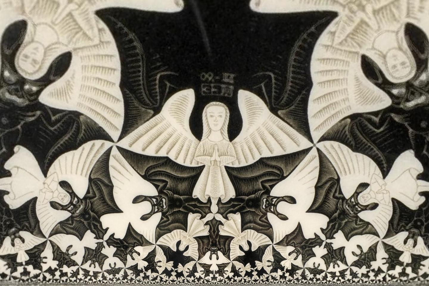
All these angels have the same size, when measured with the hyperbolic stick, that was possibly created by the hyperbolic devils, that are all of the same size as well.
 , or SL(2,R) on the half-space
  , one parameter subgroups define orbits – streamlines of the corresponding vector fields. Here are the details.
 is a path in the group SL(2,R). Suppose at
  we have
  For all
  we have
  Let
Let  be the derivative of
  Then
Then  This follows from the general identity valid for matrix functions
  with invertible
  (see e.g.
 ![\begin{equation*}\frac{d}{dt}[\det\,A(t)]=\det\,A(t)\cdot \mathrm{tr }[A(t)^{-1}\,\frac{d}{dt}A(t)].\end{equation*}](http://arkadiusz-jadczyk.eu/blog/wp-content/ql-cache/quicklatex.com-1d7e442eda5d88b039dce25a39a52ce0_l3.png "Rendered by QuickLaTeX.com")
 and
and  then
then  We have already met this property when discussing the group SU(1,1) in
  matrices with trace zero. It is denoted sl(2,R). The elements of sl(2,R) are called “generators” of the group. If
  is a generator, that is, in our case, if
  then
then  is a one-parameter subgroup of the group. That
  follows from another useful identity that can be found in Wikipedia under the term
 are matrices in sl(2,R), then
 ![Z=[X,Y]=XY-YX](http://arkadiusz-jadczyk.eu/blog/wp-content/ql-cache/quicklatex.com-5afe00e1725ed1d24f490926261d7f0b_l3.png "Rendered by QuickLaTeX.com") is also in sl(2,R) because for any two matrices
is also in sl(2,R) because for any two matrices  we have that
  Thus trace of a commutator is always zero.
 here)
here)


 maps the group SU(1,1) onto the group SL(2,R). The same transformation maps the Lie algebra su(1,1) onto the Lie algebra sl(2,R). In particular we obtain the following three generators in sl(2,R):


 on the half-plane
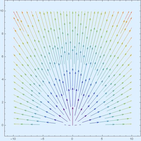
 on the half-plane
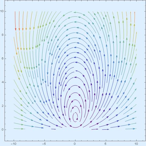
 on the half-plane
 and
and  are nilpotents (that is their squares are zero), therefore taking exponentials is easy:
 but using

 on the half-plane
  and
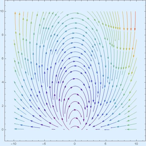
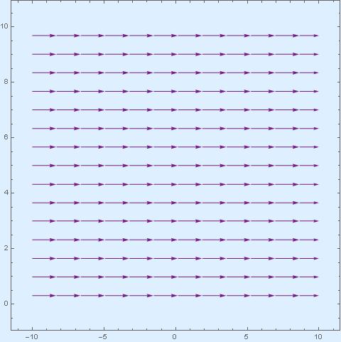
and  in the future. Their interpretation is very simple. The first one describes uniform dilation. Expanding (or contracting) in horizontal and in vertical direction at the same rate. The second one is a uniform horizontal translation. The hyperbolic geometry of the plane needs to be invariant with respect to these two kinds of transformations.
 ![[X_2',Y_+]=2Y_+.](http://arkadiusz-jadczyk.eu/blog/wp-content/ql-cache/quicklatex.com-b43d7725d1650e35efe42b8d55b8d2cc_l3.png "Rendered by QuickLaTeX.com") Therefore
Therefore  do not generate the whole sl(2,R) algebra.

 is mapped into infinity. We will not worry about this issue, as we will be mainly interested in the geometry of the interior.
 then Eq. (
 of the invariant distance on the disk. In terms of real coordinates
 will look in terms of the variables
  on the half-plane? Will it be more complicated or simpler?

 and express it in terms of
  :
: