Saturday. It was warm and sunny. Went for a bicycle raid. Working on generating the exceptional geodesic for d=0.5.
But, until that is ready, I have made another geodesic line on the three-sphere, this time for d=0.4999999 and 180 degrees rotation in 4D. Click on the image to open animation
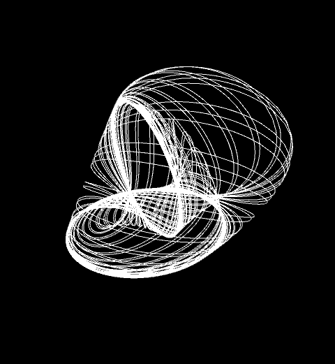
Update: I have produced the geodesic for d=1/2. Here is the result for t going from -2000 to 2000:
It is a great surprise for me. Is it really one closed line? Or, under microscope, it will split into many-many lines, very close, but with a subtle structure?
Update at 22:12
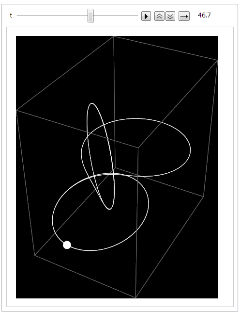
Progress. Here is one point on the trajectory (I created animation to see how it is moving)
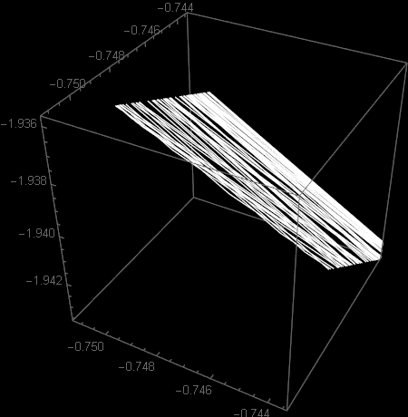
And here is zoom on the line when this point was:
The line is not a line. These are many many lines, but very close to each other.
I can’t help it. I am obsessed with geodesics.
Quoting from Encyclopedia of Mathematics:
The notion of a geodesic line (also: geodesic) is a geometric concept which is a generalization of the concept of a straight line (or a segment of a straight line) in Euclidean geometry to spaces of a more general type. The definitions of geodesic lines in various spaces depend on the particular structure (metric, line element, linear connection) on which the geometry of the particular space is based. In the geometry of spaces in which the metric is considered to be specified in advance, geodesic lines are defined as locally shortest. In spaces with a connection a geodesic line is defined as a curve for which the tangent vector field is parallel along this curve. In Riemannian and Finsler geometries, where the line element is given in advance (in other words, a metric in the tangent space at each point of the considered manifold is given), while the lengths of lines are obtained by subsequent integration, geodesic lines are defined as extremals of the length functional.
Geodesic lines were first studied by J. Bernoulli and L. Euler, who attempted to find the shortest lines on regular surfaces in Euclidean space.
The play takes place at Mr. Jourdain’s house in Paris. Jourdain is a middle-aged “bourgeois” whose father grew rich as a cloth merchant. The foolish Jourdain now has one aim in life, which is to rise above this middle-class background and be accepted as an aristocrat. To this end, he orders splendid new clothes and is very happy when the tailor’s boy mockingly addresses him as “my Lord”. He applies himself to learning the gentlemanly arts of fencing, dancing, music and philosophy, despite his age; in doing so he continually manages to make a fool of himself, to the disgust of his hired teachers. His philosophy lesson becomes a basic lesson on language in which he is surprised and delighted to learn that he has been speaking prose all his life without knowing it.
We are speaking geodesics all the time without knowing it.
On the regular two-dimensional sphere geodesics are parts of great circles
A smart ant would travel from A to B along path c, from A to C along b, and from B to C along a. These are lines as straight as only possible, that are on the surface. Geodesics on the ideal sphere are all of finite length, the maximal ones are closed, they are great circles.
But if the sphere is not so ideal, if it is a three-axial ellipsoid, even if a little bit deformed from being ideally spherical, then everything changes. Geodesics do not close, they can behave in a strange way. Again, on a small scale, they are as straight as possible, but going always “straight” we can, after long enough time, find ourselves almost everywhere. This is a difficult subject – see Geodesics on an ellipsoid.
We are not on an ellipsoid, but we are on something similar in spirit: we are on three-dimensional sphere endowed with three-axial geometry. It is the three moments of inertia that determine geometry of our After all is the whole universe of the rigid body that is rotating about its center of mass. Three parameters determine rotation matrix. Unit quaternions which we use do the same. But not all rotations are equal. Some are for the body “harder” than other, some are “easier”. This depends whether the instantaneous rotation axis is close to the one with the greatest moments of inertia, or the smallest one. Therefore also “distance” between two rotations that somehow measures “effort” exerted by the body, will depend on the direction in
I know, we will have to learn all that. But, on the other hand, it is something that should be expected. For some reason that we do not fully understand, lot fundamental equations of dynamics can be derived from “least action principle”. But least action can be translated into “shortest way”- with the appropriate definition of the distance. Therefore, perhaps, all physics can be converted into geometry, and the Nature is simply choosing always the shortest path (or, sometimes, the longest).
So, here is again the same animation, but there are more details.
You will have to click on the image to open animation in a new window. There are 91 frames. I am rotating the observer every one degree from 0 to 90 degrees. Something rather strange happens around 84 degrees. That is the extracted frame above. The animation represents one geodesic line. I mean part of it. Time goes from -2000 to 2000 (of whatever units we use). It can go from minus infinity to infinity. I have no idea how the picture would change with the extension of the length of time. Probably it would be getting denser and denser. The phenomenon here may be similar to the one exhibited by the famous chaotic Lorentz attractor.
The last post was about The final answer for the Universe in which m>1. Yet, as I see it today, it was neither complete nor final. It was a very bad approximation. It may be also that our universe is also a very bad approximation to the one that has been intended. But that is another story. I think I will return to this problem in my blogging, but now I will concentrate on the algorithm for the rotation matrix. At the same time I will make a comment how the algorithm from the last post, for the quaternions, should be improved. The fact is that I was making wrong assumptions in my mind. Making wrong assumptions, without being conscious of the fact that one is making such assumptions, that is very dangerous. Lot of bad things happens around us for this reason…. The result of wrong assumptions
So, here is the code:
The case
The solution of the Euler’s equations has two trajectories. For one with we take
(1)
while for the other one, with we take
(2)
Let
(3)
The solution of the Euler’s equations is given by
(4)
With constants and defined as
(5)
(6)
we set the phase variable as
(7)
where the Jacobi function is defined as
Let
(8)
(9)
Then the attitude matrix is given by
(10)
If you compare this with the formulas I gave yesterday, you will find the following important difference: now I am playing with signs in the constants rather than with the signs in formulas for It took me whole day to realize that this way is a better way. I was not realizing before that there is one sign in the formula for that depends on the trajectory we are taking. The constant does this job now.
In a couple of days I will also change the formulas in the quaternionic algorithm to make them universal as well.
Now, I check the modified example3. The modified initial data in init_example3.dat file are as follows:
1.0000000000D0
10.0000000000D0
-0.544332842491675D0
0.729131780907662D0
-0.414811526666455D0
1.000000000000000D0
0.000000000000000D0
0.000000000000000D0
0.000000000000000D0
1.000000000000000D0
0.000000000000000D0
0.000000000000000D0
0.000000000000000D0
1.000000000000000D0
1.000000000000000D0
1.012686988782515D0
3.306237422473038D0
5
They are the same as in the quaternionic case discussed yesterday. The initial attitude matrix is the identity matrix. We get the same I use Mathematica to calculate the transposed final
And it seems that our code is doing the same job as the Fortran code from the giants!
Yet, as I said at the beginning, it took me the whole days to figure it out why for some initial data I was in agreement, but for another initial data there was a disagreement.
There is one little plus of the code above. The coefficient in front of is fixed, and equal ! Zanna and Celledoni in their paper and in their code have complicated formulas for this coefficient. It would take some work to verify that their complicated formula simplifies to I hope I am right here….


 You do not have to know that these are geodesic lines. In
 endowed with three-axial geometry. It is the three moments of inertia
  that determine geometry of our
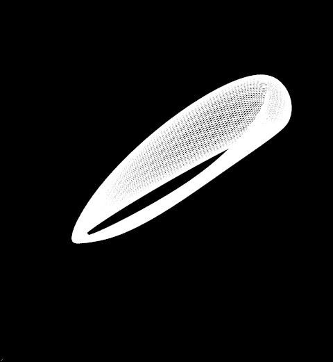


 of the Euler’s equations has two trajectories. For one with
  we take

 we take


 and
and  defined as

 as
as
 is defined as


 is given by
 rather than with the signs in formulas for
  It took me whole day to realize that this way is a better way. I was not realizing before that there is one sign in the formula for
  does this job now.
  I use Mathematica to calculate the transposed final
 is fixed, and equal
  ! Zanna and Celledoni in their paper and in their code have complicated formulas for this coefficient. It would take some work to verify that their complicated formula simplifies to


