Approaching the ultimate answer for m<1

Far out in the uncharted backwaters of the unfashionable end of the Western Spiral arm of the Galaxy lies a small unregarded yellow sun.
Orbiting this at a distance of roughly ninety-eight million miles is an utterly insignificant little blue-green planet whose ape-descended life forms are so amazingly primitive that they still think digital watches are a pretty neat idea.
This planet has—or rather had—a problem, which was this: most of the people living on it were unhappy for pretty much of the time. Many solutions were suggested for this problem, but most of these were largely concerned with the movements of small green pieces of paper, which is odd because on the whole it wasn’t the small green pieces of paper that were unhappy.
And so the problem remained; lots of the people were mean, and most of them were miserable, even the ones with digital watches.

So sets Douglas Adams the scenery in his Hitchhiker’s Guide to the Galaxy. And he is right, neither green pieces of paper nor digital watches will make us happy. But digital computers – that’s another story. Digital computer, with some patience and determination made me happy today (or I made him happy, doesn’t mater which way), and I am going now to share my happiness with you. Because there is no true happiness which is not shared happiness.

And no, I am not going to calculate the answer to the Ultimate Question of Life, the Universe and Everything. Though we will be not very far away from obtaining such an answer. But please, don’t panic!

In the last post I have perversely asked this question:

So, my guess is that the formula (23) in the paper has wrong signs. What to do?
Should I write to the authors?

Now I admit, I was not completely sincere. I was teasing, I was playing with You, the Reader. Because the truth it that months ago I discovered wrong signs in the formula (20) of this paper. So, being young and naive, I wrote to prof. Zanna announcing my discovery. Here is the reply I got:

So, we should not consider the paper as being sacred, typos sometimes happen. But software – that is something different. Software is a serious matter. The software has been thoroughly tested, so if we test our software against something that has been thoroughly tested, that will be even better than through tests of our own code!

In The Hitchhiker’s Guide to the Galaxy the answer came as forty two.

“I checked it very thoroughly,” said the computer, “and that quite definitely is the answer.

We will also check very thoroughly. Our answer will not exactly be forty two. But we will come out with a quaternion, quaternio, quatro – it can explain 4. It remains to explain the last 2.

We will be testing example four from the code 903 – you need to read a couple of previous posts if you do not know what I am talking about. Alternatively, you can download the file 903.zip, unzip it, go to the folder 903\Fortran77\Drivers, and contemplate the following three files there: driver_example4.f, init_example4.dat, out_example4.dat. All three with number four. That is what we will be doing now.

 Helsinky OH 52 - Emil ZÁTOPEK maraton
Emil Zátopek was a Czechoslovak long-distance runner best known for winning three gold medals at the 1952 Summer Olympics in Helsinki. He won gold in the 5,000 metres and 10,000 metres runs, but his final medal came when he decided at the last minute to compete in the first marathon of his life.

According to README.txt

driver_example3.f (example for FRB integration with many steps
of lenght h from 0 to Tfin, using
semi-exact methods)
To be linked with frb_step.f
driver_example4.f (Like driver_example3.f but uses quaternions)
To be linked with quat_step.f

Both examples have the body with the same moments of inertia, but initial momenta are different. So it is impossible to compare their outputs. We return to this issue later on, for now let us concentrate on example4.

The moments of inertia can be read from init_example4.dat. They are

(1)   \begin{eqnarray*} I_1&=&1.0,\\ I_2&=&1.012686988782515,\\ I_3&=&3.306237422473038 \end{eqnarray*}

So it is the same “future physics” body that we have already met in , when discussing example2.

Then comes initial angular momentum (which sometimes I call \mathbf{m} and sometimes \methbf{L}:

(2)   \begin{eqnarray*} m_1(0)&=&-0.544332842491675,\\ m_2(0)&=&0.729131780907662,\\ m_3(0)&=&-0.414811526666455. \end{eqnarray*}

As in Spinning Gulliver among giants we have

(3)   \begin{equation*} 1/I_2= 0.987472.\end{equation*}

We calculate d

    \[d =\frac{m_1(0)^2}{I_1}+\frac{m_2(0)^2}{I_2}+\frac{m_3(0)^2}{I_3}=0.873315.\]

So d<1/I_2, therefore we have m<1 case.
Now I am presenting the complete m<1 algorithm based on the method introduced in Standing on the shoulders of giants – Reboot.

The case m<1.

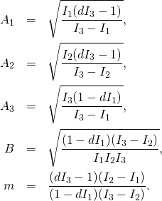
(4)   \begin{eqnarray*} A_1&=&\sqrt{\frac{I_1 (d I_3-1)}{I_3-I_1}},\\ A_2&=&\sqrt{\frac{I_2 (d I_3-1)}{I_3-I_2}},\\ A_3&=&\sqrt{\frac{I_3 (1-d I_1)}{I_3-I_1}},\\ B&=&\sqrt{\frac{(1-d I_1) (I_3-I_2)}{I_1 I_2 I_3}},\\ m&=&\frac{(d I_3-1) (I_2-I_1)}{(1-d I_1) (I_3-I_2)}. \end{eqnarray*}

The solution \mathbf{L}(t) of the Euler’s equations has two trajectories: one with L_3(t)>0 is given by

(5)   \begin{eqnarray*} L_1(t)&=&A_1\, \cn (Bt,m),\\ L_2(t)&=&A_2\, \sn (Bt,m),\\ L_3(t)&=&A_3\, \dn (Bt,m), \end{eqnarray*}

while the other one, with L_3(t)<0 is given by

(6)   \begin{eqnarray*} L_1(t)&=&-\,A_1\, \cn (Bt,m),\\ L_2(t)&=&A_2\, \sn (Bt,m),\\ L_3(t)&=&-\,A_3\, \dn (Bt,m). \end{eqnarray*}

With constants \alpha and \nu defined as

(7)   \begin{equation*} \alpha=\frac{I_3-I_1}{\sqrt{\frac{I_1(1-d I_1)(I_3-I_2)I_3}{I_2}}}, \end{equation*}

(8)   \begin{equation*} \nu=\frac{I_1-dI_1I_3}{I_3-dI_1I_3} \end{equation*}

we set the phase variable \psi(t) as

(9)   \begin{equation*} \psi(t)=\frac{t}I_1-\arctan\left((A_2/A_3)\mathrm{sd}(Bt,m)  \right)-\alpha \Pi(\nu,\am(Bt,m),m),\ \end{equation*}

where the Jacobi function \mathrm{sd} is defined as \mathrm{sd}(u,m)=\sn(u,m)/\dn(u,m).
Then the quaternionic attitude solution is given by q(t)=W(t)+\mathbf{i}X(t)+\mathbf{j}Y(t)+\mathbf{k}Z(t), with

(10)   \begin{eqnarray*} W(t)&=&\cos \frac{\psi(t)}{2}\sqrt{\frac{1+L_1(t)}{2}},\\ X(t)&=&\sin \frac{\psi(t)}{2}\sqrt{\frac{1+L_1(t)}{2}},\\ Y(t)&=&\frac{L_3(t)\cos \frac{\psi(t)}{2}+L_2(t)\sin \frac{\psi(t)}{2}}{\sqrt{2(1+L_1(t))}},\\ Z(t)&=&\frac{-L_2(t)\cos \frac{\psi(t)}{2}+L_3(t)\sin \frac{\psi(t)}{2}}{\sqrt{2(1+L_1(t))}} \end{eqnarray*}

My original intention was to verify the above with the 903 paper code using Mathematica, and, if there will be differences in the output, to fix the problems.
But now this Sunday is coming to the end, and I am getting tired. And before sleep I want to watch the second half of the movie “Master and Commander”. It fits this post:

Roger Ebert gave the film 4 stars out of 4, saying that “it achieves the epic without losing sight of the human”

Giants that stumble

User friendly means “easy to use”. We can all agree on that, I think. And it’s what we mean when we say it. So far, so good.

Except, not. When people say “easy to use”, what they REALLY mean is “easy to learn”, or “easy to use without learning”.
From What User friendly means


I am trying to make my blog user friendly. Sometimes I think I succeed. But not always. We are following giants. It is not easy. Sometimes we need to overcome our fears.

I am studying the paper and the code:

Elena Celledoni, Antonella Zanna, et al. “Algorithm 903: FRB–Fortran routines for the exact computation of free rigid body motions.” ACM Transactions on Mathematical Software, Volume 37 Issue 2, April 2010, Article No. 23, doi:10.1145/1731022.1731033

I am trying to understand it and to reproduce the results. If I am able to reproduce the results, then there is a good chance that I really understand what I am studying, and then I can share my understanding here, on the blog. Not all I am able to understand, but what to do? Sometimes I am completely lost.

Here is one such case. I am quoting one paragraph from Standing on the shoulders of giants – Reboot

I am going to use the following paper:

Elena Celledoni, Antonella Zanna, et al. “Algorithm 903: FRB–Fortran routines for the exact computation of free rigid body motions.” ACM Transactions on Mathematical Software, Volume 37 Issue 2, April 2010, Article No. 23, doi:10.1145/1731022.1731033.

The paper is only seven years old. And it has all what we need. As in Standing on the shoulders of giants we will split the attitude matrix Q into a product: Q=Q_1Q_0, but this time we will do it somewhat smarter. Celledoni and Zanna denote the angular momentum vector in the body frame using letter \mathbf{m}=(m_1,m_2,m_3), and they assume that \mathbf{m} is normalized: m=\sqrt{\mathbf{m}^2}=1. They assume, as we do, I_1<I_2<I_3, and use T to denote the kinetic energy. Let us first look at the following part of their paper (which is available here):

In the same post we introduced the matrix Q_0 that transforms vector with components (m_1,m_2,m_3) into (0,0,1). In Attitudes and Behavior we wrote it as (and I am replacing L_1(t) with m_1 etc.):

(1)   \begin{equation*}Q_0=\begin{bmatrix}1-\frac{m_1^2}{1+m_3}&-\frac{m_1m_2}{1+m_3}&-m_1\\ -\frac{m_1m_2}{1+m_3}&1-\frac{m_2^2}{1+m_3}&-m_2\\ m_1&m_2&m_3\end{bmatrix}.\end{equation*}

We have the formula unit mapping quaternions into rotation matrices (see Chiromancy in the rotation group).
If

(2)   \begin{equation*}q=W+\mathbf{i}X+\mathbf{j}Y+\mathbf{k}Z\end{equation*}

Then

(3)   \begin{equation*} R(q)=\begin{bmatrix} W^2+X^2-Y^2-Z^2&2(XY-WZ)&2(WY+XZ)\\ 2(WZ+XY)&W^2-X^2+Y^2-Z^2&2(YZ-WX)\\ 2(XZ-WY)&2(WX+YZ)&W^2-X^2-Y^2+Z^2 \end{bmatrix}, \end{equation*}

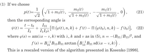
If we use the formula (21) from the paper (see image above), then

(4)   \begin{eqnarray*} W&=&\sqrt{1+m_3}/\sqrt{2},\\ X&=&\frac{m_2}{\sqrt{2(1+m_3)}},\\ Y&=&-\frac{m_1}{\sqrt{2(1+m_3)}},\\ Z&=&0. \end{eqnarray*}

Now I am using Mathematica to calculate R(q)

We obtain Q_0. Two details will catch the attention of the Reader:
In the Mathematica code I use, for instance, 1-2(Y^2+Z^2) while in the formula for R(q) I have W^2+X^2-Y^2-Z^2. But for the unit quaternion, with W^2+X^2+Y^2+Z^2, these are the same! Similarly the Mathematica code gives as the component (3,3) of the matrix

    \[\frac{1-m1^2-m2^2+m3}{1+m_3},\]

while in Q_0 we have simply m_3. But again, with m_1^2+m_2^2+m_3^2=1, the Reader will easily check that these are the same!
So it seems that we are progressing with our understanding of the language and the science of giants! Success. Therefore we must not stop! We must continue!
After the case m>1 Celledoni and Zanna move to the case of m<1:

So, if we understand it correctly, for m<1 we should replace Q_0 matrix with the new one, constructed the same way as before, but with the third axis being replaced by the first. The quaternion that implements such a rotation, according to the formula (23) from the paper, should be given by

(5)   \begin{eqnarray*} W&=&\sqrt{1+m_1}/\sqrt{2},\\ X&=&0,\\ Y&=&-\frac{m_3}{\sqrt{2(1+m_1)}},\\ Z&=&\frac{m_2}{\sqrt{2(1+m_1)}}.\\ \end{eqnarray*}

I calculate R(q) for this quaternion, and I get …. mess. Certainly not the matrix that acting on (m_1,m_2,m_3) would give (1,0,0). So, something is wrong! I am trying to compare the formulas in the paper with those in the Fortran code. But then I am getting confused even more. For the case m>1 the code has these lines:

APPP = 1.0D0 + EM30
APP = SQRT(APPP)
ADUE=SQRT(2.0D0)
Q2(1) = APP/ADUE
Q2(4) = -0.0D0
Q2(2) = -Q2(1)*EM20/APPP
Q2(3) = Q2(1)*EM10/APPP

We recognize that Q2(1) is our W=\sqrt{1+m_3}/\sqrt{2} in Eqs. (\label{eq{wxyz3}), Q2(4) is our Z. EM10,EM20,EM30 is probably our m_1,m_2,m_3. If so, then Q2(2) is minus our X and Q2(3) is minus our Y. I have no idea why there are minuses, but there are there!

What about the case m<1? The code has these lines:

APPP = 1.0D0 + EM10
APP = SQRT(APPP)
ADUE=SQRT(2.0D0)
Q2(1) = APP/ADUE
Q2(2) = 0.0D0
Q2(3) = -Q2(1)*EM30/APPP
Q2(4) = Q2(1)*EM20/APPP

Again we recognize Q2(1) as our W=\sqrt{1+m_1}/\sqrt{2} we recognize Q2(2) as X=0. But now the signs in Q2(2) and Q2(3) agree with those in the paper. Something weird is going on. So, as an experiment I change the signs in formula (23):

(6)   \begin{eqnarray*} W&=&\sqrt{1+m_1}/\sqrt{2},\\ X&=&0,\\ Y&=&\frac{m_3}{\sqrt{2(1+m_1)}},\\ Z&=&-\frac{m_2}{\sqrt{2(1+m_1)}}.\\ \end{eqnarray*}

So that, consistently, the two signs in the paper are opposite to those in the code. Now R(q) gives what it is supposed to do: rotation matrix that transforms (m_1,m_2,m_3) into (1,0,0).

So, my guess is that the formula (23) in the paper has wrong signs. What to do?
Should I write to the authors? My thinking goes into the direction: it would be of no use.
The paper is 7 years old. In fact the preprint tells me that the work has been essentially finished in 2008. Now the authors are working on a different project, they have other things to do than worrying about signs in a formula. Perhaps the formula is wrong, so what? Who cares? No one is reading paper anyway. Scientists write papers in order to document that they were busy with something, to show that they are experts, to get new grants, to be quoted. Anyway intelligent reader should be able to fix typos. It should even be advised to make some errors. Fixing someone’s errors takes our time, true. But, on the other hand, what a wonderful opportunity to think and to verify that we really understand the subject! Finding errors in pear reviewed papers gives us reassurance that referees in these papers, as a rule, do not pay attention to the question as to whether a given paper is correct or incorrect. It should simply give a strong impression that it is correct.. That is all.
True, some authors take mistakes in their published works seriously. I like to quote this particular very good example: ERRATA TO ANALYSIS, MANIFOLDS AND PHYSICS. PART I, the monograph by Yvonne Choquet-Bruhat and Cecile DeWitt-Morette, is 11 pages long. With all kinds of errors corrected, including correction to wrong proofs. That is life.

So, let us continue. We take what is good. We correct what can be corrected. And we move forward.

I was going to make this post about the case m>1 – to give the complete algorithm. But somehow I got deflected, I stumbled. I will recover in the next post.

Attitudes and Behavior

To quote from Wikipedia:

Method

LaPiere travelled round America with a Chinese couple, expecting to meet discrimination as a result of anti Chinese feeling. At the time prejudice against Asians was widespread and there were no laws against racial discrimination. They visited 67 hotels and 184 restaurants. Six months later, after their return, all the establishments they had visited were sent a letter, asking whether they would accept Chinese guests.

Results

They were only refused at one of the establishments they visited, and were generally treated very politely. Of the 128 establishments which responded to the letter, 91% said they were not willing to accept Chinese guests.

Conclusion

Attitudes do not always predict behavior. Cognitive and affective components of attitudes are not necessarily expressed in behavior.

The LaPiere’s study shows that the cognitive and affective components of attitudes (e.g. disliking Chinese people) do not necessarily coincide with behavior (e.g. serving them).

Very clever are these psychologists. But we are discussing attitude matrix of the free rigid body. We did not quite finish in the last post with the case m>1. I will finish it here. First we have to go back to Standing on the shoulders of giants – Reboot, where we have introduced the new matrix Q0(t). I will write it here in a slightly different form:

(1)   \begin{equation*}\begin{bmatrix}1-\frac{L_1(t)^2}{1+L_3(t)}&-\frac{L_1(t)L_2(t)}{1+L_3(t)}&-L_1(t)\\ -\frac{L_1(t)L_2(t)}{1+L_3(t)}&1-\frac{L_2(t)^2}{1+L_3(t)}&-L_2(t)\\ L_1(t)&L_2(t)&L_3(t)\end{bmatrix}.\end{equation*}

Assuming that L_1^2+L_2^2+L_3^2=1, it is a simple exercise to check that both formulas give the same result. Given the matrix Q_0 we can use the same method that we have used before in Taming the T-handle, find the equation for \psi, and solve it. This time solution involves elliptic function: \mathrm{sd}=\sn/\dn. Here is the formula I have obtained using computer algebra software (I am doing copy and paste from Mathematica):

(2)   \begin{multline*}\psi(t)=\frac{(\text{I3}-\text{I1}) \Pi \left(\frac{\text{I3}-d \text{I1} \text{I3}}{\text{I1}-d \text{I1} \text{I3}};\left.\text{am}\left(\left.t \sqrt{\frac{(\text{I2}-\text{I1}) (d \text{I3}-1)}{\text{I1} \text{I2} \text{I3}}}\right|m\right)\right|m\right)}{\sqrt{\frac{\text{I1} \text{I3} (d \text{I3}-1) (\text{I2}-\text{I1})}{\text{I2}}}}\\-\tan ^{-1}\left(\frac{\text{sd}\left(t \sqrt{\frac{(\text{I2}-\text{I1}) (d \text{I3}-1)}{\text{I1} \text{I2} \text{I3}}}|\frac{(1-d \text{I1}) (\text{I3}-\text{I2})}{(\text{I2}-\text{I1}) (d \text{I3}-1)}\right)}{\sqrt{-\frac{\text{I1} (d \text{I3}-1) (\text{I1}-\text{I2})}{\text{I2} (d \text{I1}-1) (\text{I1}-\text{I3})}}}\right)+\frac{t}{\text{I3}};\end{multline*}

Then, in order to obtain the attitude matrix, we do the same as before. And I will continue and explain in the next post. With the new form of the attitude we will obtain exactly the same behavior as with the previous attitude. Yet for quaternions the new attitude will be much better!