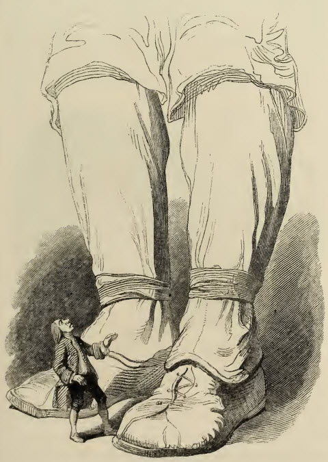
I am following giants. At least I am trying. For Gulliver it was not so funny to be in the land of giants:
Certainly Jonathan Swift was a giant of literature. Another giant, among those that I am trying to learn from, is G. K. Chesterton:
Gilbert Keith Chesterton was a giant in many ways. His six-feet-two inches and corpulent figure made him a physical giant but it was the extent and diversity of his writings that made him a giant in the field of literature and theology. He proved to be a great defender of the Catholic faith and crossed swords with the likes of George Bernard Shaw on theological matters yet they remained friends, and Shaw called him ‘a man of colossal genius’
Well well, we really should listen to giants:
The human race, to which so many of my readers belong, has been playing at children’s games from the beginning, and will probably do it till the end, which is a nuisance for the few people who grow up. And one of the games to which it is most attached is called “Keep to–morrow dark,” and which is also named (by the rustics in Shropshire, I have no doubt) “Cheat the Prophet.” The players listen very carefully and respectfully to all that the clever men have to say about what is to happen in the next generation. The players then wait until all the clever men are dead, and bury them nicely. They then go and do something else. That is all. For a race of simple tastes, however, it is great fun.
For human beings, being children, have the childish wilfulness and the childish secrecy. And they never have from the beginning of the world done what the wise men have seen to be inevitable. They stoned the false prophets, it is said; but they could have stoned true prophets with a greater and juster enjoyment. Individually, men may present a more or less rational appearance, eating, sleeping, and scheming. But humanity as a whole is changeful, mystical, fickle, delightful. Men are men, but Man is a woman.
Hmmm…. In my last note, Standing on the shoulders of giants – Reboot,
I started the discussion of one paper by two ladies, Elena Celledoni, Antonella Zanna, et al. “Algorithm 903: FRB–Fortran routines for the exact computation of free rigid body motions.” ACM Transactions on Mathematical Software, Volume 37 Issue 2, April 2010, Article No. 23, doi:10.1145/1731022.1731033. But I did not connect in any way to the content of their paper. I am presenting here a long series of posts about rotations of free rigid bodies, but it is in the spirit of playing games like children do. While the ladies with their paper are serious. I remember what the Bible says:

Yes, it is time to put away childish things or, better, to learn how to talk like an adult to adults. So, let’s do it.
There is the paper, and there is the code. Both can be downloaded and examined. More important is the code. Paper may contain typos. Papers often do. Paper you read. Code you run. There is the code, and there are examples of its application. This is a serious matter. We should be able to check if are able to reproduce the results. Let’s take example 2. Here are initial data that we will try to understand:
1.0000000000D0
10.0000000000D0
-0.609860759302936D0
0.761660947972381D0
0.218957654801698D0
1.000000000000000D0
0.000000000000000D0
0.000000000000000D0
0.000000000000000D0
1.000000000000000D0
0.000000000000000D0
0.000000000000000D0
0.000000000000000D0
1.000000000000000D0
1.000000000000000D0
1.012686988782515D0
3.306237422473038D0
First we have time step. Then we have time. Time is t=10.
Then we have initial angular momentum (in the body frame)
(1) 
I checked and we get indeed norm 1.
Then we have the initial attitude matrix  – the identity matrix.
The last three lines are the moments of inertia:
(2) 
The fact that  tells us that mathematicians (our two ladies) have more imagination than physicists. At present we do not have materials that would provide such data (for positive mass densities we should always have
  ) but in the near future physics and technology may easily move to the place where mathematicians are already today. It is reassuring that already today we can predict and model the behavior of such exotic materials.
Let us calculate the parameter  (the ratio of doubled kinetic energy to the square of angular momentum)
![\[d =\frac{m_1(0)^2}{I_1}+\frac{m_2(0)^2}{I_2}+\frac{m_3(0)^2}{I_3}=0.95929.\]](http://arkadiusz-jadczyk.eu/blog/wp-content/ql-cache/quicklatex.com-255480b90194e4bdbebc26c8be9e19ad_l3.png "Rendered by QuickLaTeX.com")
Since  we have the case when
  I will use the Mathematica code from our children games:
A1 = Sqrt[I1*(d*I3 – 1)/(I3 – I1)]
A2 = Sqrt[I2*(d*I3 – 1)/(I3 – I2)]
A3 = Sqrt[I3*(1 – d*I1)/(I3 – I1)]
B = Sqrt[(1 – d*I1)*(I3 – I2)/(I1*I2*I3)]
m = ((d*I3 – 1)*(I2 – I1))/((1 – d*I1)*(I3 – I2))
Using these formulas we get:
(3) 
We see that  as we expected.
We will use the Mathematica code from our children games:

Looking at the initial angular momentum data we see that  is positive, therefore we can stay with the formulas above, we do not need to change signs of two of the angular momenta inside the code.
Now, what do we do with initial angular momenta? In our code we need to find the time  at which we obtain these values. From that time on we will have to run the code for t=10. So our problem is to solve the following equations:
(4) 
We do not have to worry about , because it is already determined by  and
and 
We know that
![\[\cn(B t_0, m)=\cos \am(B t_0,m),\]](http://arkadiusz-jadczyk.eu/blog/wp-content/ql-cache/quicklatex.com-325bb9dcd4e6eecd37c5d64ef4ceaa0b_l3.png "Rendered by QuickLaTeX.com")
![\[\sn(B t_0,m)=\sin \am(B t_0,m).\]](http://arkadiusz-jadczyk.eu/blog/wp-content/ql-cache/quicklatex.com-c3ee20a7f6ccb38c8ebacef61bba5485_l3.png "Rendered by QuickLaTeX.com")
Thus, using Mathematica ArcTan function:
![\[\am(B t_0,m)=ArcTan[m_1(0)/A_1,m_2(0)/A_2].\]](http://arkadiusz-jadczyk.eu/blog/wp-content/ql-cache/quicklatex.com-a74ac0564dfed88daffd65b02f1ac05c_l3.png "Rendered by QuickLaTeX.com")
I use Mathematica and get
![\[\am(B t_0,m)=2.25039.\]](http://arkadiusz-jadczyk.eu/blog/wp-content/ql-cache/quicklatex.com-46a1564f1db48d022d31fd929e032e0d_l3.png "Rendered by QuickLaTeX.com")
But  is the inverse function of EllipticF. So I calculate
![\[t_0=EllipticF[2.25039,m]/B=14.9607.\]](http://arkadiusz-jadczyk.eu/blog/wp-content/ql-cache/quicklatex.com-3ab920f9fbd7ead2a315e56f991e82f7_l3.png "Rendered by QuickLaTeX.com")
So we know  Knowing I use the code above to calculate
  We get
(5) 
In the example from the code we have  therefore to get what they get I need to calculate
  at
at 
We use the Mathematica code above to get:
(6) 
To make comparison easier with the results obtained by Celledoni and Zanna, let us transpose the matrix, because they write the output columnwise.
(7) 
And here is the result from the code of Celledoni and Zanna at the end of out_example3.dat file:
0.7511853766362874
-0.1659110385305551
-0.6389006630310473
-0.1233163682782040
-0.9861296978083955
0.1110913696692821
-0.6484702022780026
-4.6633029105353817E-03
-0.7612257551892809
It seems that we can now speak the language of adults as well. This encouraging and we can continue our adventure.
The Mathematica notebook with these calculations can be downloaded from here.
Being at peace with matrices, we can move to more dangerous quaternions.


 Antonella Zanna
 into a product:
  but this time we will do it somewhat smarter. Celledoni and Zanna denote the angular momentum vector in the body frame using letter
  and they assume that
  is normalized:
  They assume, as we do,
  and use
  to denote the kinetic energy. Let us first look at the following part of their paper (which is available
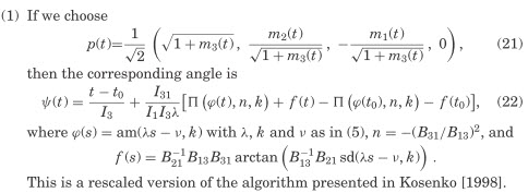
 using the notation in my posts. That means “high energy regime”.
 Suppose we construct a matrix
  that transforms
  into
into  . The attitude matrix
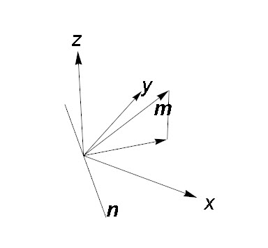
 plane. Draw a line
  on
on  between
 Its projection on
  Orthogonal vector in
  (to check orthogonality calculate scalar product), So the normalized vector
 ![\[\mathbf{n}=(\frac{m_2}{m_p}, -\frac{m_1}{m_p},0),\]](http://arkadiusz-jadczyk.eu/blog/wp-content/ql-cache/quicklatex.com-bf4a8a65edb4f56f68ea76f8d08d619b_l3.png "Rendered by QuickLaTeX.com")
![\[m_p=\sqrt{m_1^2+m_2^2}.\]](http://arkadiusz-jadczyk.eu/blog/wp-content/ql-cache/quicklatex.com-5d53a1df1f449812587d51ec4f773a87_l3.png "Rendered by QuickLaTeX.com")
 Its sinus is
![\[R=I+\sin\theta\, W(\vec{n})+(1-\cos\theta)\,W(\vec{n})^2,\]](http://arkadiusz-jadczyk.eu/blog/wp-content/ql-cache/quicklatex.com-2d29b03988528678a18fb8be1c0658f9_l3.png "Rendered by QuickLaTeX.com")


 acting on
  vector gives
  is invariant under
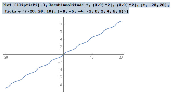
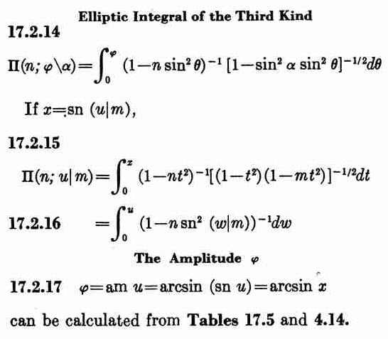
 solving the differential equation for the attitude matrix involves EllipticPi function. As I have explained it in

 but such a conversion is possible only in the domain where
  can be inverted. We can do it easily for sufficiently small values of
  but not necessarily for values that contain several quarter-periods.