New wine in new bottles

In my recent post I was presenting new formulas for the attitude matrix, different from those of a month ago. And I did not explain in detail how I got them, and why they look like being in disagreement with the previous ones. This caused a legitimate concern from Bjab, when he noticed the apparent disagreement. And indeed putting new wine into old bottles would lead to a trouble.

Mar 2:21 No man also seweth a piece of new cloth on an old garment: else the new piece that filled it up taketh away from the old, and the rent is made worse.
Mar 2:22 And no man putteth new wine into old bottles: else the new wine doth burst the bottles, and the wine is spilled, and the bottles will be marred: but new wine must be put into new bottles.


What we did is this: we poured new wine into new bottles. And here is how it is done.

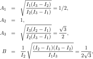
We consider free rigid body with normalized (unit length) angular momentum vector, and the doubled kinetic energy equal to d=1/I_2. Euler’s equations can be then solved explicitly and we choose the following solution:

(1)   \begin{eqnarray*} A_1&=&\sqrt{\frac{I_1(I_3-I_2)}{I_2(I_3-I_1)}}=1/2,\\ A_2&=&1,\\ A_3&=&\sqrt{\frac{I_3(I_2-I_1)}{I_2(I_3-I_1)}}=\frac{\sqrt{3}}{2},\\ B&=&\frac{1}{I_2}\,\sqrt{\frac{(I_2-I_1)(I_3-I_2)}{I_1I_3}}=\frac{1}{2\sqrt{3}},\\ \end{eqnarray*}
(2)   \begin{eqnarray*} L_1(t)&=& A_1\,\mathrm{sech }(B t),\\ L_2(t)&=&A_2\,\tanh( B t),\\ L_3(t)&=&A_3\,\mathrm{sech }(B t), \end{eqnarray*}

where \mathrm{sech }(x)=1/\cosh(x).
We will need the angular velocity vector with components

(3)   \begin{equation*}\Omega_i(t)=\frac{L_i(t)}{I_i}.\end{equation*}

We want to solve now the differential equation for the attitude matrix Q(t):

(4)   \begin{equation*}\frac{dQ(t)}{dt}=Q(t)W(t),\end{equation*}

where

(5)   \begin{equation*}W(t)=\begin{bmatrix}0&-\Omega_3(t)&\Omega_2(t)\\\Omega_3(t)&0&-\Omega_1(t)\\-\Omega_2(t)&\Omega_1(t)&0\end{bmatrix}.\end{equation*}

The strategy is this: We seek the solution of the form Q(t)=Q_2(t)Q_1(t), where Q_1(t) is a certain matrix cleverly constructed out of L_i(t), and Q_2(t) is a simple rotation matrix by some angle \psi(t).
There are two methods: old one, and new one.

The old method.

In the old method, as used for instance in Taming the T-handle continued (we use now Q_1,Q_2 instead of Q_0,Q_1 there), we set:

(6)   \begin{equation*} L_p(t)=\sqrt{L_1(t)^2+L_2(t)^2},\end{equation*}

(7)   \begin{equation*}Q_1(t)=\begin{bmatrix}\frac{L_1(t)L_3(t)}{L_p(t)}&\frac{L_2(t)L_3(t)}{L_p(t)}&-L_p(t)\\-\frac{L_2(t)}{L_p(t)}&\frac{L_1(t)}{L_p(t)}&0\\L_1(t)&L_2(t)&L_3(t)\end{bmatrix},\end{equation*}

(8)   \begin{equation*}Q_2(t)=\begin{bmatrix}\cos\psi(t)&-\sin\psi(t)&0\\\sin\psi(t)&\cos\psi(t)&0\\0&0&1\end{bmatrix}.\end{equation*}

Then we solve for \psi(t):

(9)   \begin{equation*}\psi(t)=\frac{t}{I_2}+\arctan\left( \sqrt{\frac{(I_2-I_1)I_3}{I_1(I_3-I_2)}}\tanh\sqrt{\frac{(I_2-I_1)(I_3-I_2)}{I_1I_2^2I_3}}t  \right).\end{equation*}

The new method.

(10)   \begin{equation*} Q_1(t) =\begin{bmatrix} L_1(t)& L_2(t)& L_3(t)\\-L_2(t)&     1 - \frac{L_2(t)^2}{1 + L_1(t)}& -\frac{L_2(t) L_3(t)}{1 + L_1(t)}\\  -L_3(t)& -\frac{L_2(t) L_3(t)}{1 + L_1(t)}&     1 - \frac{L_3(t)^2}{1 + L_1(t)},\end{bmatrix} \end{equation*}

(11)   \begin{equation*} Q_2(t)=\begin{bmatrix}  1 & 0 & 0 \\  0 & \cos \psi (t) & -\sin \psi (t) \\  0 & \sin \psi (t) & \cos \psi (t) \\ \end{bmatrix}. \end{equation*}

(12)   \begin{equation*} \psi(t)=\frac{t}{I_2}+2\arctan\left(\delta \tanh(B t/2)\right), \end{equation*}

where

(13)   \begin{equation*}\delta&=&\frac{\sqrt{I_2(I_3-I_1)}-\sqrt{I_1(I_3-I_2)}}{\sqrt{I_3(I_2-I_1)}}.\end{equation*}

Comparing old and new wines

In both cases we get a solution of the attitude differential equation (4). But these are different solutions. If Q(t) is a solution, and if R is a fixed rotation matrix of determinant one, then RQ(t) is another solution. This is the same body rotating, but observed from two different laboratory frames.
Let Q_{old}(t) and Q_{new}(t) be the two solutions, one obtained with the old, the other one with the new method.
With some little algebra it can be verified that Q_{new}(0)=RQ_{old}(0), where

(14)   \begin{equation*}R=\begin{bmatrix}0&0&1\\0&1&0\\-1&0&0\end{bmatrix}.\end{equation*}

.
Therefore for all t

(15)   \begin{equation*}Q_{new}(t)=R Q_{old}(t).\end{equation*}

I verified it numerically. The above comparison was for rotation matrices. For quaternions it is similar, though the quaternion case deserves a comment. I will give it in another note.

Update: Mathematica notebook verifying Eq. (15) numerically is available here.

Attitude matrix for m<1

The last post was about The final answer for the Universe in which m>1. Yet, as I see it today, it was neither complete nor final. It was a very bad approximation. It may be also that our universe is also a very bad approximation to the one that has been intended. But that is another story. I think I will return to this problem in my blogging, but now I will concentrate on the algorithm for the rotation matrix. At the same time I will make a comment how the algorithm from the last post, for the quaternions, should be improved. The fact is that I was making wrong assumptions in my mind. Making wrong assumptions, without being conscious of the fact that one is making such assumptions, that is very dangerous. Lot of bad things happens around us for this reason….

Plane crash
The result of wrong assumptions

So, here is the code:

The case m<1.
The solution \mathbf{L}(t) of the Euler’s equations has two trajectories. For one with L_3(t)>0 we take

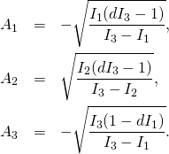
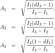
(1)   \begin{eqnarray*} A_1&=&\sqrt{\frac{I_1 (d I_3-1)}{I_3-I_1}},\\ A_2&=&\sqrt{\frac{I_2 (d I_3-1)}{I_3-I_2}},\\ A_3&=&\sqrt{\frac{I_3 (1-d I_1)}{I_3-I_1}},\\ \end{eqnarray*}

while for the other one, with L_3(t)<0 we take

(2)   \begin{eqnarray*} A_1&=&-\sqrt{\frac{I_1 (d I_3-1)}{I_3-I_1}},\\ A_2&=&\sqrt{\frac{I_2 (d I_3-1)}{I_3-I_2}},\\ A_3&=&-\sqrt{\frac{I_3 (1-d I_1)}{I_3-I_1}}.\\ \end{eqnarray*}

Let

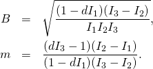
(3)   \begin{eqnarray*} B&=&\sqrt{\frac{(1-d I_1) (I_3-I_2)}{I_1 I_2 I_3}},\\ m&=&\frac{(d I_3-1) (I_2-I_1)}{(1-d I_1) (I_3-I_2)}. \end{eqnarray*}

The solution \mathbf{L}(t) of the Euler’s equations is given by

(4)   \begin{eqnarray*} L_1(t)&=&A_1\, \cn (Bt,m),\\ L_2(t)&=&A_2\, \sn (Bt,m),\\ L_3(t)&=&A_3\, \dn (Bt,m), \end{eqnarray*}

With constants \alpha and \nu defined as

(5)   \begin{equation*} \alpha=\frac{I_3-I_1}{\sqrt{\frac{I_1(1-d I_1)(I_3-I_2)I_3}{I_2}}}, \end{equation*}

(6)   \begin{equation*} \nu=\frac{I_1-dI_1I_3}{I_3-dI_1I_3} \end{equation*}

we set the phase variable \psi(t) as

(7)   \begin{equation*} \psi(t)=\frac{t}I_1+\arctan\left((A_2/A_3)\mathrm{sd}(Bt,m)  \right)-\alpha \Pi(\nu,\am(Bt,m),m),\ \end{equation*}

where the Jacobi function \mathrm{sd} is defined as \mathrm{sd}(u,m)=\sn(u,m)/\dn(u,m).
Let

(8)   \begin{equation*} \begin{equation*} Q_1(t) =\begin{bmatrix} L_1(t)& L_2(t)& L_3(t)\\-L_2(t)&     1 - \frac{L_2(t)^2}{1 + L_1(t)}& -\frac{L_2(t) L_3(t)}{1 + L_1(t)}\\  -L_3(t)& -\frac{L_2(t) L_3(t)}{1 + L_1(t)}&     1 - \frac{L_3(t)^2}{1 + L_1(t)},\end{bmatrix} \end{equation*}

(9)   \begin{equation*} Q_2(t)=\begin{bmatrix}  1 & 0 & 0 \\  0 & \cos \psi (t) & -\sin \psi (t) \\  0 & \sin \psi (t) & \cos \psi (t) \\ \end{bmatrix}. \end{equation*}

Then the attitude matrix Q(t) is given by

(10)   \begin{equation*}Q(t)=Q_2(t)Q_1(t).\end{equation*}

If you compare this with the formulas I gave yesterday, you will find the following important difference: now I am playing with signs in the constants A_1,A_3 rather than with the signs in formulas for L_1(t),L_3(t). It took me whole day to realize that this way is a better way. I was not realizing before that there is one sign in the formula for \psi(t) that depends on the trajectory we are taking. The constant A_2/A_3 does this job now.

In a couple of days I will also change the formulas in the quaternionic algorithm to make them universal as well.

Now, I check the modified example3. The modified initial data in init_example3.dat file are as follows:
1.0000000000D0
10.0000000000D0
-0.544332842491675D0
0.729131780907662D0
-0.414811526666455D0
1.000000000000000D0
0.000000000000000D0
0.000000000000000D0
0.000000000000000D0
1.000000000000000D0
0.000000000000000D0
0.000000000000000D0
0.000000000000000D0
1.000000000000000D0
1.000000000000000D0
1.012686988782515D0
3.306237422473038D0
5
They are the same as in the quaternionic case discussed yesterday. The initial attitude matrix is the identity matrix. We get the same t_0. I use Mathematica to calculate the transposed final Q

Transpose[Inverse[Q[t0]].Q[t0 + 10.0]]
{{0.0656754, 0.550118, -0.832501}, {0.995487, 0.0211483,
0.0925082}, {0.0684964, -0.834819, -0.546246}}

We compare it with the Fortran output from 903 code:

0.0656754297
0.55011776
-0.832500564
0.995487311
0.0211482921
0.0925081752
0.0684963551
-0.834819262
-0.546246326

And it seems that our code is doing the same job as the Fortran code from the giants!
Yet, as I said at the beginning, it took me the whole days to figure it out why for some initial data I was in agreement, but for another initial data there was a disagreement.

There is one little plus of the code above. The coefficient in front of \arctan is fixed, and equal 1.! Zanna and Celledoni in their paper and in their code have complicated formulas for this coefficient. It would take some work to verify that their complicated formula simplifies to 1. I hope I am right here….

The final answer for the Universe in which m<1

This is not an independent post or note or whatever. It is a continuation. In fact it is the continuation of Approaching the ultimate answer for m<1. We have approached enough. We are ready.

There was a moment’s expectant pause while panels slowly came to life on the front of the console. Lights flashed on and off experimentally and settled down into a businesslike pattern. A soft low hum came from the communication channel.
“Good morning,” said Deep Thought at last.
“Er … good morning, O Deep Thought,” said Loonquawl nervously, “do you have … er, that is …”
“An answer for you?” interrupted Deep Thought majestically. “Yes. I have.”
The two men shivered with expectancy. Their waiting had not been in vain.
“There really is one?” breathed Phouchg.
“There really is one,” confirmed Deep Thought.

Douglas Adams, The Hitchhiker’s Guide to the Galaxy

We did not get to the answer yesterday, but today is the day. We will be using the formulas from the last post. Here they are again, repeated for your convenience:

The case m<1.

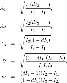
(1)   \begin{eqnarray*} A_1&=&\sqrt{\frac{I_1 (d I_3-1)}{I_3-I_1}},\\ A_2&=&\sqrt{\frac{I_2 (d I_3-1)}{I_3-I_2}},\\ A_3&=&\sqrt{\frac{I_3 (1-d I_1)}{I_3-I_1}},\\ B&=&\sqrt{\frac{(1-d I_1) (I_3-I_2)}{I_1 I_2 I_3}},\\ m&=&\frac{(d I_3-1) (I_2-I_1)}{(1-d I_1) (I_3-I_2)}. \end{eqnarray*}

The solution \mathbf{L}(t) of the Euler’s equations has two trajectories: one with L_3(t)>0 is given by

(2)   \begin{eqnarray*} L_1(t)&=&A_1\, \cn (Bt,m),\\ L_2(t)&=&A_2\, \sn (Bt,m),\\ L_3(t)&=&A_3\, \dn (Bt,m), \end{eqnarray*}

while the other one, with L_3(t)<0 is given by

(3)   \begin{eqnarray*} L_1(t)&=&-\,A_1\, \cn (Bt,m),\\ L_2(t)&=&A_2\, \sn (Bt,m),\\ L_3(t)&=&-\,A_3\, \dn (Bt,m). \end{eqnarray*}

With constants \alpha and \nu defined as

(4)   \begin{equation*} \alpha=\frac{I_3-I_1}{\sqrt{\frac{I_1(1-d I_1)(I_3-I_2)I_3}{I_2}}}, \end{equation*}

(5)   \begin{equation*} \nu=\frac{I_1-dI_1I_3}{I_3-dI_1I_3} \end{equation*}

we set the phase variable \psi(t) as

(6)   \begin{equation*} \psi(t)=\frac{t}I_1-\arctan\left((A_2/A_3)\mathrm{sd}(Bt,m)  \right)-\alpha \Pi(\nu,\am(Bt,m),m),\ \end{equation*}

where the Jacobi function \mathrm{sd} is defined as \mathrm{sd}(u,m)=\sn(u,m)/\dn(u,m).
Then the quaternionic attitude solution is given by q(t)=W(t)+\mathbf{i}X(t)+\mathbf{j}Y(t)+\mathbf{k}Z(t), with

(7)   \begin{eqnarray*} W(t)&=&\cos \frac{\psi(t)}{2}\sqrt{\frac{1+L_1(t)}{2}},\\ X(t)&=&\sin \frac{\psi(t)}{2}\sqrt{\frac{1+L_1(t)}{2}},\\ Y(t)&=&\frac{L_3(t)\cos \frac{\psi(t)}{2}+L_2(t)\sin \frac{\psi(t)}{2}}{\sqrt{2(1+L_1(t))}},\\ Z(t)&=&\frac{-L_2(t)\cos \frac{\psi(t)}{2}+L_3(t)\sin \frac{\psi(t)}{2}}{\sqrt{2(1+L_1(t))}} \end{eqnarray*}

We consider Example Four with

(8)   \begin{eqnarray*} I_1&=&1.0,\\ I_2&=&1.012686988782515,\\ I_3&=&3.306237422473038 \end{eqnarray*}

(9)   \begin{eqnarray*} m_1(0)&=&-0.544332842491675,\\ m_2(0)&=&0.729131780907662,\\ m_3(0)&=&-0.414811526666455. \end{eqnarray*}

m_3(0) is negative, the therefore we take option as in Eq. 3). We calculate t_0 that reproduces the initial angular momenta. The method is known from the previous posts:

(10)   \begin{equation*}am=\arctan(-m_1(0)/A_1,m_2(0)/A_2)=0.925158,\end{equation*}

(11)   \begin{equation*}t_0=\mathrm{EllipticF}(am,m)=3.17243.\end{equation*}

So we have t_0. At t=t_0 our angular momentum is the same as angular momentum in example 4 at t=0. We calculate q_0=q(t_0) from Eq'(7)

    \[q_0=W(t_0)+X(t_0)\,\mathbf{i}+Y(t_0)\,\mathbf{j}+Z(t_0)\,\mathbf{k},\]

(12)   \begin{eqnarray*} W(t_0)&=&0.435964,\\ X(t_0)&=&0.194343,\\ Y(t_0)&=&-0.0858987,\\ Z(t_0)&=-&0.874521 \end{eqnarray*}

thus

(13)   \begin{equation*}q_0=0.435964+0.194343\,\mathbf{i}-0.0858987\,\mathbf{j}-0.874521\,\mathbf{k}.\end{equation*}

We verify that we have indeed a unit quaternion:

    \[||q_0||^2=W(t_0)^2+X(t_0)^2+Y(t_0)^2+Z(t_0)^2=1.0.\]

Thus the inverse quaternion is the same as conjugated one:

    \[q_0^{-1}=0.435964-0.194343\,\mathbf{i}+0.0858987\,\mathbf{j}+0.874521\,\mathbf{k}.\]

In the Example 4 the initial quaternion, at t=0 is 1. Therefore in order for our solution to reproduce the initial data of the example we set

(14)   \begin{equation*}\tilde{q}(t)=q_0^{-1}\,q(t+t_0).\end{equation*}

The final time in Example 4 is t=10. Therefore we calculate

(15)   \begin{equation*}\tilde{q}(10)=q_0^{-1}q(10+t_0),\end{equation*}

where the multiplication is the quaternion multiplication.
Calculated with Mathematica the answer is

(16)   \begin{eqnarray*} W&=&=-0.36762,\\ X&=&-0.630629,\\ Y&=&-0.612723,\\ Z&=&0.302874. \end{eqnarray*}

The result from the Fortran code in the file out_example4.dat is

-0.3676198430772359
-0.6306293413288832
-0.6127232632258010
0.3028737154869889


It seems that therefore that we have obtained the ultimate answer. At least for quaternions. We need to get it also for rotation matrices. So the saga will continue.