Standing on the shoulders of giants may be good, even very-very good. But at the same time it can be very dangerous. First of all it is a dangerous balancing act. It is easy to fall.
But what if the giant gets a hiccup? Or stumble? You may die. Or someone can die because of aftershocks.
In Standing on the shoulders of giants I quoted two papers that I used in working out my computer simulations of Dzhanibekov’s effect. These were
Ramses van Zon, Jeremy Schofield, “Numerical implementation of the exact dynamics of free rigid bodies“, J. Comput. Phys. 225, 145-164 (2007)
and
Celledoni, Elena; Zanna, Antonella.E Celledoni, F Fassò, N Säfström, A Zanna, The exact computation of the free rigid body motion and its use in splitting methods, SIAM Journal on Scientific Computing 30 (4), 2084-2112 (2008)
The algorithms were working smoothly. But recently I decided to use quaternions instead of rotation matrices. And in recent post Introducing geodesics, I have presented a little animation:
It looks impressive, but if we pay attention to details, we see something strange:

We have a nice curly trajectory, but there are also strange straight line spikes. On animation they are, perhaps, harmless. But if something like this happens with the software controlling the flight of airplanes, space rockets or satellites – people may die. There is a BUG in the algorithm. Yes, I did stay on shoulders of giants, but perhaps they were not the right giants for my aims? And indeed this happens. The method I used is not appropriate for working with quaternions.
That is why I have to do the reboot, and look for another giant. Here is my giant:
 Antonella Zanna, professor of Mathematics, University of Bergen, specialty Numerical Analysis/Geometric Integration.
I am going to use the following paper:
Elena Celledoni, Antonella Zanna, et al. “Algorithm 903: FRB–Fortran routines for the exact computation of free rigid body motions.” ACM Transactions on Mathematical Software, Volume 37 Issue 2, April 2010, Article No. 23, doi:10.1145/1731022.1731033.
The paper is only seven years old. And it has all what we need. As in Standing on the shoulders of giants we will split the attitude matrix  into a product:
  but this time we will do it somewhat smarter. Celledoni and Zanna denote the angular momentum vector in the body frame using letter
  and they assume that
  is normalized:
  They assume, as we do,
  and use
  to denote the kinetic energy. Let us first look at the following part of their paper (which is available here):
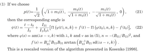
Though it is not very important, I must say that it is very nice of the two authors that they acknowledge Kosenko. I was trying to study Kosenko’s paper, but I gave up not being able to understand it. Then wen notice that the case considered is that of  using the notation in my posts. That means “high energy regime”.
The angular momentum is constant (fixed) in the laboratory frame owing to the conservation of angular momentum. Suppose we orient the laboratory frame so that its z axis is oriented along the angular momentum vector. Then, in the laboratory frame angular momentum has coordinates  Suppose we construct a matrix
  that transforms
  into
into  . The attitude matrix transforms vector components in the body frame into their components in the laboratory frame. In particular it transforms into . Therefore,if we write the matrix must transform into itself. Therefore must be a rotation about the third axis, that is it is of the form:
(1) 
All of that we have discussed already in Standing on the shoulders of giants. But now we are going to choose differently.
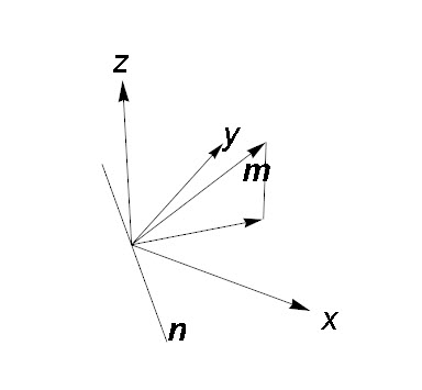
So suppose we have vector of unit length. What would be the most natural way of constructing a rotation matrix that rotates into ? Simple. Project vertically onto  plane. Draw a line
  on plane that is perpendicular to the projection. Rotate about this line by the angle
  between and
Let us now do the calculations. Vector has components  Its projection on plane has components
  Orthogonal vector in plane has components
  (to check orthogonality calculate scalar product), So the normalized vector has components
![\[\mathbf{n}=(\frac{m_2}{m_p}, -\frac{m_1}{m_p},0),\]](http://arkadiusz-jadczyk.eu/blog/wp-content/ql-cache/quicklatex.com-bf4a8a65edb4f56f68ea76f8d08d619b_l3.png "Rendered by QuickLaTeX.com")
where
![\[m_p=\sqrt{m_1^2+m_2^2}.\]](http://arkadiusz-jadczyk.eu/blog/wp-content/ql-cache/quicklatex.com-5d53a1df1f449812587d51ec4f773a87_l3.png "Rendered by QuickLaTeX.com")
The cosinus of the angle is  Its sinus is
In Spin – we know that we do not know we have derived a general formula for a rotation about an angle about axis defined by a unit vector :
![\[R=I+\sin\theta\, W(\vec{n})+(1-\cos\theta)\,W(\vec{n})^2,\]](http://arkadiusz-jadczyk.eu/blog/wp-content/ql-cache/quicklatex.com-2d29b03988528678a18fb8be1c0658f9_l3.png "Rendered by QuickLaTeX.com")
where for any vector 
(2) 
Applying the formula to our case, simple algebra leads to:
(3) 
We can easily check that indeed is an orthogonal matrix with determinant 1,  acting on
  vector gives One can also check that the vector
  is invariant under – as it should be as it is on the rotation axis. REDUCE program that checks it all is here.
At this point we have to make a break. It is not yet clear what is the relation of my to the paper quoted, what is the difference between this and the old version, and why is this version better?
We will continue climbing on the shoulders of giants in the following notes. But, please, remember, Standing on shoulders of giants (like “Nobel Prize Winner” Obama), is risky:


 with components
  are
are
 are principal moments of inertia. We assume that our spinning body is asymmetric, therefore
  Perhaps it is worthwhile to mention that physics of ordinary materials requires that all three numbers are strictly positive, and that
  I have my pet rigid body that is essentially flat, with
  It looks as on the picture below
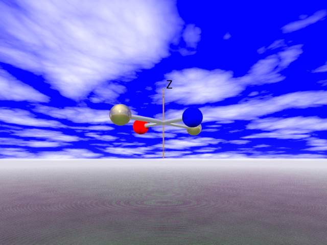
 They deserve a separate study.
 that maps coordinates in the rotating frame to coordinates in the laboratory frame.
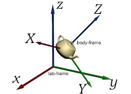
 be an orthonormal frame corotating with the body, and aligned with its principal axes, and let
  be an inertial laboratory frame, both centered at the center of mass of the body. The two frames are related by time-dependent orthogonal matrix

 is denoted by
 are coordinates of a fixed point in the body, then its coordinates in the laboratory system change in time:


 that associates a matrix to every vector. In fact it associates an antisymmetric matrix. The association has the property that is easy to verify: for every vector
  we have
![\[W(\vec{v})\,\vec{w}=\vec{v}\times\vec{w}.\]](http://arkadiusz-jadczyk.eu/blog/wp-content/ql-cache/quicklatex.com-2251427987114047af49cc8e4cbb7bf7_l3.png "Rendered by QuickLaTeX.com")
 is the same as taking cross product with vector
  That such an association should exist should be not a surprise. Taking cross-product with a fixed vector is a linear operation, and every linear operation on vectors is implemented by a matrix. However many students who learn about cross products,
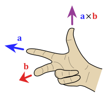
 of determinant one we have:

 that represents the angular momentum vector in the laboratory frame, and
  that represents the same vector in the body frame. Our matrix
  by definition, connects the two representations (see Eq. (
![\[\boldsymbol{\omega}=Q\,\boldsymbol{\Omega}.\]](http://arkadiusz-jadczyk.eu/blog/wp-content/ql-cache/quicklatex.com-fc1aa035220c91d2701888f1c908ff30_l3.png "Rendered by QuickLaTeX.com")
![\[W(\boldsymbol{\omega})Q=W(Q\boldsymbol{\Omega})Q=Q\,W(\boldsymbol{\Omega})Q^t\,Q=Q\,W(\boldsymbol{\Omega}),\]](http://arkadiusz-jadczyk.eu/blog/wp-content/ql-cache/quicklatex.com-67fb083fab044417706ed07f48386312_l3.png "Rendered by QuickLaTeX.com")
 where
where  is a constant. The solution of the attitude matrix equation is
![\[\frac{dM(t)}{dt}=M(t)X,\]](http://arkadiusz-jadczyk.eu/blog/wp-content/ql-cache/quicklatex.com-39e8257063c231f6550bf2c49d7de3a5_l3.png "Rendered by QuickLaTeX.com")
 is a constant (i.e. time independent) matrix, we can verify that
  is a solution. In fact, it is the unique solution with the initial data
  To prove it, one would have to expand
  into power series, take care about the convergence of the infinite series (no care needed, it is absolutely convergent), and then differentiate term by term. Let us take it for granted that is the case. In the quote from the other post above I used the letters
  but, as in the remark above, we are supposed to adjust the meaning to the context. For the matrix
  so the solution with the property
  is
is  which, because
  If so, the right side of the Euler’s equations is automatically zero. Therefore any constant vector
  units of time. As noticed above the solution of the attitude equation is
  Therefore
  is the rotation matrix that describes the rotation about the axis in the direction
  . We have already used this fact before, but now it was a good place for recollecting.
 of our free asymmetric top, in the body frame, satisfies
 satisfy Euler’s equations, and we change the sign of any two of them, then we will have another solution of Euler’s equations. The same concerns angular momentum components
  That is because either both of these changed components are on the right, then the product of two minuses cancels out giving plus, or one is on the left and one is on the right, and again the changes cancel out.
 and the code for the solution has these lines:
 and the function
  is always non-negative. That is why the point moves in the northern hemisphere. If we change the signs of the first two components of the angular momentum vector, that is equaivalent to the rotation by 180 degrees around the vertical axis. The motion will be the same, but the point will be on the opposite side of the curve.
 whose components are functions of time, but the equations do not contain time
  is a solution, then
  is another solution, for any
  We can move the origin of the time axis to any point in time. Let us have a look at the table from
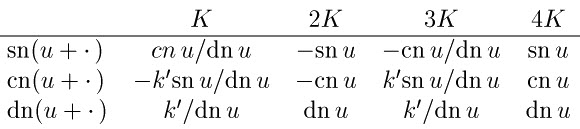
 is the same as changing the signs of the first two components. And this is the same as shifting the point on the trajectory by half of its period, which is
 is non-positive.


 is larger than 1:
  One has to be careful now, because the definitions of the Jacobi functions for
  are tricky (see


 , that is
  can be written as


