From “The Crack in the Cosmic Egg: Challenging Constructs of Mind and Reality”, by Joseph Chilton Pearce (a must read!):
My neighbor was “seized and changed” somewhere in his final year of doctoral studies in topology. The structure of his mind, and his resulting world, were never again the same as that of non-mathematicians. He lived in a world of mathematical spaces. He loved to figure the spaces of knots, the kind you tie, though I could not relate his marvelous figurings to my shoelace world. He tried to show me, in beautifully-diagrammed hieroglyphics, how he could remove an egg from an intact shell through mathematical four-space. In my naive concreteness, frustrated that I had no ears to hear or eyes to see, I wanted him to apply his four-space miracle to a common hen’s egg. But my friend’s world was cerebral, his eggs those rare cosmic ones found in the inner land of thought, and his frustration at my blindness was as great as my own.
There is an eloquent madness in topology, but from that strange brotherhood’s abstractions lunar modules have been built. From their four-spaced absurdities have come real ships for spaces other than our own. The mythos leads the logos. The language of fantasy goes before the language of fact.
The physics and mathematics of asymmetric rigid top is harder than topology (see Asymmetric Spinning Top – The Hardest Concept To Grasp In Physics). It has its own egg’s tricks. A static egg has been critically analyzed in Racket about tennis racket. Then I started to move to the movies in The Flipping Top Movie that they will not show you in the movie theaters!.
“The mythos leads the logos.” But we did not yet finish with the mythos. So, let us contemplate these two animations produced by Mathematica software. Here they are:

And here is the code:
d = 0.501;
I1 = 1; I2 = 2; I3 = 3;
A1 = Sqrt[I1*(d*I3 – 1)/(I3 – I1)];
A2 = Sqrt[I2*(d*I3 – 1)/(I3 – I2)];
A3 = Sqrt[I3*(1 – d*I1)/(I3 – I1)];
B = Sqrt[(1 – d*I1)*(I3 – I2)/(I1*I2*I3)];
m = ((d*I3 – 1)*(I2 – I1))/((1 – d*I1)*(I3 – I2))
m1[t_] = A1*JacobiCN[B*t, m];
m2[t_] = A2*JacobiSN[B*t, m];
m3[t_] = A3*JacobiDN[B*t, m];
If[m < 1, tf = N[4*EllipticK[m]/B],
tf = N[4*EllipticK[1/m]/(B*Sqrt[m])]];
g = x^2 + y^2 + z^2 – 1;
h = x^2/I1 + y^2/I2 + z^2/I3 – d;
cp = ContourPlot3D[{h == 0, g == 0}, {x, -1.5, 1.5}, {y, -1.5,
1.5}, {z, -1.8, 1.8},
MeshFunctions -> {Function[{x, y, z, f}, h – g]},
MeshStyle -> {{Thick, Blue}}, Mesh -> {{0}},
ContourStyle ->
Directive[Orange, Opacity[0.5], Specularity[White, 30]],
PlotPoints -> 40, BoxRatios -> Automatic, Background -> Black,
Axes -> True,
AxesLabel -> {“\!\(\*SubscriptBox[\(L\), \(1\)]\)”,
“\!\(\*SubscriptBox[\(L\), \(2\)]\)”,
“\!\(\*SubscriptBox[\(L\), \(3\)]\)”}, AxesStyle -> White]
plot2b = Table[
Show[{cp,
Graphics3D[{Yellow,Sphere[{m1[a], m2[a], m3[a]}, 0.05]}]}], {a, -tf/2,
tf/2 – tf/10, tf/20}];
Export[“C:/egg0501.gif”, plot2b,
AnimationRepetitions -> Infinity, ImageSize -> {240, 240}]
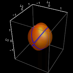
For the first animation the parameter $d$ is set to $d=0.499.$ What do we see? How is what we see in the animations related to the code? At the beginning of the code we see $I1 = 1; I2 = 2; I3 = 3;$ These are the characteristics of my olympic champion flipping and making vaults top. Girls do it their way
My rigid body does it even better. My rigid body has as its principal moments of inertia the first three prime numbers!. You can’t beat it! Of course there will be people that will attempt to discredit it, like: “Ït is using doping.” Which is not true at all! Or: “Number 1 is not a prime number”. They do not know history of mathematics. Read here from Wolfram MathWorld, Prime Number: “The number 1 is a special case which is considered neither prime nor composite (Wells 1986, p. 31). Although the number 1 used to be considered a prime (Goldbach 1742; Lehmer 1909, 1914; Hardy and Wright 1979, p. 11; Gardner 1984, pp. 86-87; Sloane and Plouffe 1995, p. 33; Hardy 1999, p. 46)…”. It is clear that it is the primest of all primes!
So, my spinning rigid body wins all competitions. Let me recall it explicitly from the previous post:
Now let us see these moments of inertia in a spectacular action of freely rotating in space. Not just rotating! Rotating and then flipping.
Click on the image to open the animation in a new window. Depending on your connection it may take a while. The size is almost 1 MB. You will see the flips. But why? What causes these flips?
The code above provides explicit solutions for the Euler’s equations for this champion. Look at the first animation. You see a white moving point. It moves along a curve in the northern hemisphere. It belongs to the family curves discussed in The Flipping Top Movie that they will not show you in the movie theaters!
Except that the path on the animation is more elongated than on the image above. But why the northern hemisphere? Why not the southern one? It looks like racial discrimination!
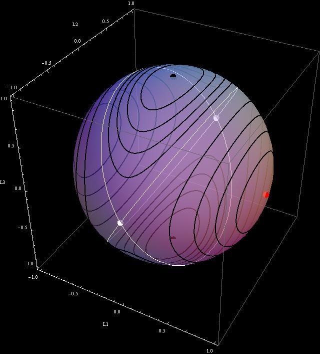
Or the second animation. The yellow point moves only on path on the right. Not on the left. Why should leftist movements be neglected?
These are valid questions. Perhaps the Readers will try to answer them?
* Right now I am aware of the fact that this blog has two active readers.

 are the components of the angular velocity vector in the body frame, while
  are the three
  where
where  has components
  Although we do not know
  (it needs to be found through solving differential equations), we know that it is an orthogonal matrix. And orthogonal matrix preserves the length of the vector. Since the components of the vector
  are constants, also its length is a constant. But the length of
  and the length squared
  of
of 
 the doubled
 :
:![\[\frac{d}{dt}\,2E=2(I_1\Omega_1\dot{\Omega_1}+I_2\Omega_2\dot{\Omega_2}+I_3\Omega_3\dot{\Omega_3}).\]](http://arkadiusz-jadczyk.eu/blog/wp-content/ql-cache/quicklatex.com-b3d495d6abddaf4dfb277c844f48c43e_l3.png "Rendered by QuickLaTeX.com")


 of the angular momentum given by Eq. (
![\[ I_12E=I_1(I_1\Omega_1^2+I_2\Omega_2^2+I_3\Omega_3^2)=I_1^2\Omega_1^2+I_1I_2\Omega_2^2+I_1I_3\Omega_3^2\leq L^2.\]](http://arkadiusz-jadczyk.eu/blog/wp-content/ql-cache/quicklatex.com-a3a87ae5ce21926c99c88cfed085f6f1_l3.png "Rendered by QuickLaTeX.com")
![\[ I_32E\geq L^2.\]](http://arkadiusz-jadczyk.eu/blog/wp-content/ql-cache/quicklatex.com-7e5ee5d8a0a01cd237e1c786a1f6430c_l3.png "Rendered by QuickLaTeX.com")
 defined by

 that we have derived in “
 . Our guess is that
  is proportional to
  We do not know whether to assume
  proportional to
  or to
or to  ? Let us try
  proportional to
 such that the Euler’s equation are satisfied automatically, given

 be an orthonormal frame corotating with the body, and aligned with its principal axes, and let
  be an inertial laboratory frame, both centered at the center of mass of the body. The two frames are related by time-dependent orthogonal matrix

 is denoted by
 are coordinates of a fixed point in the body, then its coordinates in the laboratory system change in time:

 is orthogonal,
  therefore, by differentiating, the matrix
  is antisymmetric. Every antisymmetric
  matrix
  can be written as

![\[ \frac{dQ(t)}{dt}Q(t)^{-1}=W(\boldsymbol{\omega}(t)),\]](http://arkadiusz-jadczyk.eu/blog/wp-content/ql-cache/quicklatex.com-e1d9b73168a8ba5dc3cf3485e0d9b60a_l3.png "Rendered by QuickLaTeX.com")

 is equivalent to taking the crossproduct with vector
 is the angular velocity vector in the laboratory frame.
 the body representative of the angular velocity vector
  where we skip the time dependence, with components


![\[W(\Omega)\mathbf{v}=\Omega\times\mathbf{v}\]](http://arkadiusz-jadczyk.eu/blog/wp-content/ql-cache/quicklatex.com-566ad7dfbf8172cfad2ece9ed8124f82_l3.png "Rendered by QuickLaTeX.com")
 and
and  If
If ![\[ Q\Omega\times Q\mathbf{v}=Q(\Omega\times\mathbf{v}). \]](http://arkadiusz-jadczyk.eu/blog/wp-content/ql-cache/quicklatex.com-eff7632b8414cfffdc1ee024090b1399_l3.png "Rendered by QuickLaTeX.com")
![\[W(Q\Omega)Q\mathbf{v}=QW(\Omega)\mathbf{v}.\]](http://arkadiusz-jadczyk.eu/blog/wp-content/ql-cache/quicklatex.com-9448f2d5d36abf4a7791ba332f0284bc_l3.png "Rendered by QuickLaTeX.com")
 then
then![\[W(Q\Omega)\mathbf{w}=QW(\Omega)Q^t\mathbf{w}.\]](http://arkadiusz-jadczyk.eu/blog/wp-content/ql-cache/quicklatex.com-fd6dea6cd6be226fe4cee71dd6e61d53_l3.png "Rendered by QuickLaTeX.com")
 can be arbitrary, we get
![\[W(Q\Omega)=QW(\Omega)Q^t.\]](http://arkadiusz-jadczyk.eu/blog/wp-content/ql-cache/quicklatex.com-8b8c914942e6ab25f91e5ddf2c7f0301_l3.png "Rendered by QuickLaTeX.com")

 In the body frame the inertia tensor
  is diagonal
  The angular momentum vector
![\[L_1=I_1\Omega_1,\,L_2=I_2\Omega_2,\,L_3=I_3\Omega_3.\]](http://arkadiusz-jadczyk.eu/blog/wp-content/ql-cache/quicklatex.com-c49b6f49b55594bd0f73b8528d946302_l3.png "Rendered by QuickLaTeX.com")
 is the product of mass
  and velocity
  and angular velocity components
  The expression for the angular momentum in the body frame is very simple, but the law of conservation of the angular momentum refers to angular momentum vector in the laboratory frame. The transition from the body to the laboratory frame is implemented by the attitude matrix
![\[ \dot{Q}(t)\mathbf{L}(t)+Q(t)\frac{d}{dt}\mathbf{L}(t)=0.\label{eq:c2}\]](http://arkadiusz-jadczyk.eu/blog/wp-content/ql-cache/quicklatex.com-5b5e458f26fb7375d5bd3518fb7d524f_l3.png "Rendered by QuickLaTeX.com")
 therefore Eq. (??) reduces to
![\[ Q(t)W(\boldsymbol{\Omega})\mathbf{L}(t)+Q(t)\frac{d}{dt}\mathbf{L}(t)=0.\label{eq:c2a}\]](http://arkadiusz-jadczyk.eu/blog/wp-content/ql-cache/quicklatex.com-7b7c6af5d3c2a5fc72b10e8e5385f648_l3.png "Rendered by QuickLaTeX.com")
 from the left:
![\[ W(\boldsymbol{\Omega})\mathbf{L}(t)+\frac{d}{dt}\mathbf{L}(t)=0.\label{eq:c2a}.\]](http://arkadiusz-jadczyk.eu/blog/wp-content/ql-cache/quicklatex.com-22be7be7c1eae500267fa4d57806c5cb_l3.png "Rendered by QuickLaTeX.com")

![\[ \frac{d}{dt}\mathbf{L}(t)=\mathbf{L}\times\boldsymbol{\Omega}.\label{eq:c2b}.\]](http://arkadiusz-jadczyk.eu/blog/wp-content/ql-cache/quicklatex.com-403e9c9478db295b499cbb807ea0eb50_l3.png "Rendered by QuickLaTeX.com")
 we arrive at
 Here they are written in terms of


