Yesterday, while thinking about Dzhanibekov effect, gyroscopes and elliptic functions, I checked my mailbox and read the following email from one of the readers:
Dear Ark,
Can you write about Kozyriev mirrors in your future posts? Rossiya 1 did a documentary awhile ago still available here:
Kozyrev Mirrors_Breakthrough into the Future – (english subtitles)
What are your thoughts of what might be going on in these experiments? Do the Kozyriev mirror experiments have to do with time traveling and accessing the information field? Why a “concave” mirror or cylinder? What is special about this shape and the materials used? Would it be detrimental for people to experiment with these mirrors? Any scientific or informal thoughts on this subject will be most welcomed.
The truth is: in my imagination gyroscopes and Kozyrev’s mirrors are completely different subjects. But then I asked myself: or aren’t they?
After small search I have downloaded from the Internet THE SCIENCE OF TORSION, GYROSCOPES AND PROPULSION. It starts with
“SOMETHING IS MISSING IN THE SCIENCE OF SPINNING SYSTEMS”
My critical article on Shipov’s “4D gyroscopes” is mentioned there, but the works and ideas of Kozyrev are also mentioned.
Wikipedia article on Kozyrev with his mirrors quotes “Akimov, A.E., Shipov, G. I., Torsion fields and their experimental manifestations, 1996” – the subject closely related to the “unconventional physics” of spinning objects. So, perhaps at some deeper level the two subjects are closely related? With this in mind I will have to read what is available about research done with Kozyrev’s mirrors. At present I know next to nothing, and what I once knew I have mostly forgotten. But I will keep it in mind, study, and in the future return the strange properties of space, vacuum, structured aether and Kozyrev mirrors. For now, however, I need to finish what I have started – nonlinear mathematical pendulum. Today we will discuss the expressions for its period.
Pendulum period: 
In the previous post Rescaled Jacobi amplitude – general solution for the mathematical pendulum, we have derived a general formula for time evolution of a nonlinear mathematical pendulum
(1) 
where  is the ratio
  of maximal potential energy to maximal kinetic energy, and
  where
where  is the gravitational acceleration, and
  is the length of the pendulum.
The inequality means that the pendulum has sufficient kinetic energy to swing full circles. Lets us recall the graph of the amplitude function 
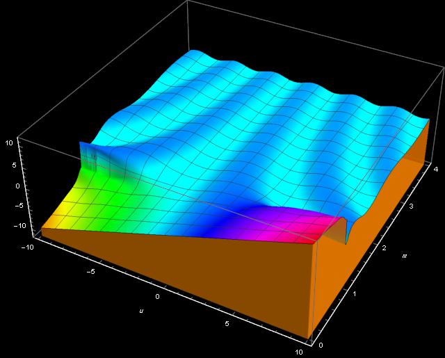
For the value of grows from left to right. That is clear: the angle  constantly increases. But when it riches
  the pendulum, in fact makes a full circle. Therefore the period
  of our pendulum is calculated from the formula
(2) 
We recall from Jacobi amplitude- realism or cubism that  is the inverse function of
  the incomplete elliptic integral of the first kind given by (see also Wikipedia: Elliptic integral)
(3) 
Therefore Eq. (2) is equivalent to
![\[ \frac{\omega T} {k}= F(\pi,m).\]](http://arkadiusz-jadczyk.eu/blog/wp-content/ql-cache/quicklatex.com-8fcaeecb1efdeea6d5e9a6ceac81c334_l3.png "Rendered by QuickLaTeX.com")
The function under integral in Eq. (3) has the symmetry property that tells us that  The value
  is usually given the name: the complete elliptic integral of the first kind, and it is often denoted with the capital letter
  Thus we obtain:
(4) 
The case of  is uninteresting, as it means either the pendulum of zero potential, or of infinite kinetic energy. In the case of
  we have, in fact, two possible solutions. One is with constant,
  That is very unstable, like a pencil that stands on its tip. There is also second solution, one given by our formula with
  The motion is non-periodic, there is just one flip all around the circle, and it takes infinite time.
Pendulum period: 
For we have to return to the definition of the amplitude function – Eqs (1),(2) in Jacobi elliptic cn and dn:
(5) 
We can see from the graph above that for the function  oscillates periodically. Since, taking into account simplification of multiplying and dividing by
  , we get
![\[\mathrm{am}(\frac{\omega t} {k},m)=\arcsin\left(\frac{1}{k}\mathrm{sn}(\omega t,1/m)\right),\]](http://arkadiusz-jadczyk.eu/blog/wp-content/ql-cache/quicklatex.com-bfa593f2fc268997b85344d3990e7dcb_l3.png "Rendered by QuickLaTeX.com")
it follows that the period of is the same as the period of the function  and it is the same as the period of the function
It is therefore given by the formula
![\[\omega T=F(2\pi,1/m),\]](http://arkadiusz-jadczyk.eu/blog/wp-content/ql-cache/quicklatex.com-24f38485e983f1d45f219e9157fac789_l3.png "Rendered by QuickLaTeX.com")
therefore

For very small oscillation (very small kinetic energies)  is very large and
  is close to zero. The integrand in the definition of
  can be replaced by the constant
  , so that, for very large ,
  Therefore
  can be replaced by
  and Eq. (6) reduces to
(7) 
This is the standard formula for the linear pendulum with small oscillation. It was known to Galileo.


 and the length of the pendulum
  . Usually it is denoted by
  but we will use
 changes with time
  We will use the dot to denote time derivative of
 ![\[\dot{\theta}=d\theta(t)/dt.\]](http://arkadiusz-jadczyk.eu/blog/wp-content/ql-cache/quicklatex.com-b7208dda67b628d381f523d78a1f7da5_l3.png "Rendered by QuickLaTeX.com")
 of the pendulum is
  , therefore the kinetic energy
  is
is![\[E_k=\frac{\mu V^2}{2}=\frac{\mu l^2\dot{\theta}^2}{2}.\]](http://arkadiusz-jadczyk.eu/blog/wp-content/ql-cache/quicklatex.com-b4be9ab4282a94b9065cca4790f863aa_l3.png "Rendered by QuickLaTeX.com")
 the height of the mass with respect to the lowest level, we have
![\[ h= l(1-\cos\theta).\]](http://arkadiusz-jadczyk.eu/blog/wp-content/ql-cache/quicklatex.com-ee9bb4288c5d6099e4041d0687d96682_l3.png "Rendered by QuickLaTeX.com")
 we have
  for
for  we have
  Here it is useful to introduce the half-angle
  We know from trigonometry that
 ![\[ 1-\cos \theta =2 \sin^2 \theta/2.\]](http://arkadiusz-jadczyk.eu/blog/wp-content/ql-cache/quicklatex.com-f74d6db171470d890074ca404a42cd32_l3.png "Rendered by QuickLaTeX.com")

 is
is  that is
 is at the bottom, for
  at the point. Maximal potential energy
  is at the top:
 When this ratio is
  there will be not enough kinetic energy to rise the swinging mass to the top, and the pendulum will oscillate back and forth. But when the ratio
  then
then![\[ m=k^2\stackrel{df}{=}\frac{E_{p,max}}{E_{k,max}}.\]](http://arkadiusz-jadczyk.eu/blog/wp-content/ql-cache/quicklatex.com-7986d7ac7fcc05c2cad18f240a39f3cd_l3.png "Rendered by QuickLaTeX.com")

![\[ E_k+E_p=E_{k,max}.\]](http://arkadiusz-jadczyk.eu/blog/wp-content/ql-cache/quicklatex.com-673d60ddf072d7e5d475ce4721dc695e_l3.png "Rendered by QuickLaTeX.com")
 with the corresponding expressions derived above we get
 therefore
 defined as

 in front of
  on the left. But this can be easily accomodated by changing the time scale. With
 ![\[\frac{k^2}{\omega^2}\left(\frac{d}{dt}\,\mathrm{am}(\frac{\omega t}{k},m)\right)^2=\left(\mathrm{am}'(\frac{\omega t}{k},m)\right)^2=1-m\,\sin^2(\mathrm{am}(\frac{\omega t}{k},m)).\]](http://arkadiusz-jadczyk.eu/blog/wp-content/ql-cache/quicklatex.com-c3e716595de5093862f7847e0667a67f_l3.png "Rendered by QuickLaTeX.com")


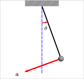
 Here, with this picture, we are assuming the the initial push given to the pendulum is not too large. Thus the pendulum, when swinging to the right, can reach at most the point B. The current angle of the pendulum is
  the maximal angle is
  Later on we will deal with the case of a pendulum with enough energy to complete full circles, but for now let us restrict our attention to “tamed pendulums”.


