Nowadays mathematics is almost everywhere. To know some cool mathematics (or mathematician) is nowadays sexy.
Therefore I am helping you here, on this blog, to have better relations in your lives. Just looking at the equations can already make you feel better. When you look for a little at Euler’s equations, you will sleep better. That is why today I recall some of these pretty formulas from the dynamics of spinning bodies.
Repetitio est mater studiorum – repetition is the mother of study/

It is not that climbing up is difficult. It is not. We can take stairs. But it takeS time. And that is what we are going to do now: take time, do it easy way. Enjoying happy sliding down afterwards.
The two essential ingredients af the asymmetric top spinning in zero gravity are:
- Euler’s equations
- Attitude matrix equations
Euler equations, written in terms of the angular momentum vector  with components
  are
are
(1) 
 are principal moments of inertia. We assume that our spinning body is asymmetric, therefore are all different from each other, and we will order them as
  Perhaps it is worthwhile to mention that physics of ordinary materials requires that all three numbers are strictly positive, and that
  I have my pet rigid body that is essentially flat, with
  It looks as on the picture below
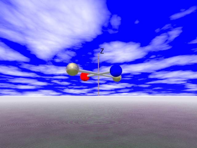
It is kind of simple but it shows all the nontrivial behavior that a rigid body can have.
Remark: As noted by Bjab in the discussion of this post, the sentence above is incorrect. At the other end of the spectrum of rigid body shapes there are one-dimensional objects. These are flying rods with  They deserve a separate study.
But that is not important now. What is important is that the components are the components of the angular momentum vector with respect to the noninertial frame that rotates with the body. Its components with respect to the inertial laboratory frame are constant in time. This is “conservation of angular momentum”- one of the most fundamental “laws” of classical mechanics. Why such a law holds, or at least approximately holds, in our Universe is not known. Physicists and philosophers are debating about “the origin of inertia”. Some say that “because of space”, some say “because of distant parallelism”, some other say “because of distant matter”. We will not worry about these problems now. We have our laboratory inertial frame, we have frame rotating with the body, and we have rotation matrix  that maps coordinates in the rotating frame to coordinates in the laboratory frame.
Recall from Angular momentum
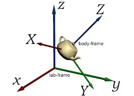
Let  be an orthonormal frame corotating with the body, and aligned with its principal axes, and let
  be an inertial laboratory frame, both centered at the center of mass of the body. The two frames are related by time-dependent orthogonal matrix
(2) 
The inverse of  is denoted by
(3) 
and it is often called the attitude matrix. For a rotating body, if  are coordinates of a fixed point in the body, then its coordinates in the laboratory system change in time:
(4) 
Matrix satisfies differential equation that is essentially nothing more than the definition of the angular velocity vector:
(5) 
thus


A couple of comments are due at this point. First of all a careful Reader will notice that in Angular momentum we had
(9) 
(10) 
What is going on?
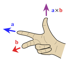
Several things at once. First we have the map  that associates a matrix to every vector. In fact it associates an antisymmetric matrix. The association has the property that is easy to verify: for every vector
  we have
![\[W(\vec{v})\,\vec{w}=\vec{v}\times\vec{w}.\]](http://arkadiusz-jadczyk.eu/blog/wp-content/ql-cache/quicklatex.com-2251427987114047af49cc8e4cbb7bf7_l3.png "Rendered by QuickLaTeX.com")
Acting with the matrix  is the same as taking cross product with vector
  That such an association should exist should be not a surprise. Taking cross-product with a fixed vector is a linear operation, and every linear operation on vectors is implemented by a matrix. However many students who learn about cross products,
do not learn about their relation to antisymmetric matrices and bivectors. And many students that are learning about matrices, operations with them, eigenvalues and eigenvectors, do not learn about cross-product of vectors. Perhaps because the cross-product is particular to 3D?
Anyway, we have this association, and this association has a very nice property of “covariance”: for every orthogonal matrix  of determinant one we have:

That is a very important and very useful property. It can be equivalently expressed as the “covariance of the cross-product”
(12) 
But equivalent expression does not replace the proof, and to prove it needs a bunch of simple but lengthy algebraic calculations and taking into account the definitions of cross-product and determinant. It can be easily done with any computer algebra software. I skip it now.
The second thing is the difference between  that represents the angular momentum vector in the laboratory frame, and
  that represents the same vector in the body frame. Our matrix
  by definition, connects the two representations (see Eq. (4) above, but now we skip the time-dependence):
![\[\boldsymbol{\omega}=Q\,\boldsymbol{\Omega}.\]](http://arkadiusz-jadczyk.eu/blog/wp-content/ql-cache/quicklatex.com-fc1aa035220c91d2701888f1c908ff30_l3.png "Rendered by QuickLaTeX.com")
Now, going back to Eq. (9), we have (again we skip the time dependence)
![\[W(\boldsymbol{\omega})Q=W(Q\boldsymbol{\Omega})Q=Q\,W(\boldsymbol{\Omega})Q^t\,Q=Q\,W(\boldsymbol{\Omega}),\]](http://arkadiusz-jadczyk.eu/blog/wp-content/ql-cache/quicklatex.com-67fb083fab044417706ed07f48386312_l3.png "Rendered by QuickLaTeX.com")
which solves our puzzle.
Remark: Above we have used and to distinguish between numerical representation of the same vector with respect to two different frames. But when there is no possibility of a confusion, we can denote a vector by any convenient letter whatsoever.
Let us see how the above recollection of facts can be applied. In Towards the road less traveled with spin there was the following statement:
The vertical z-axis is the natural axis to try to spin the thing. Imagine our top is floating in space, in zero gravity. We take the z-axis between our fingers, and spin the device. If our hand is not shaking too much, our top will nicely spin about the z-axis. This is the most stable axis for spinning.
The corresponding solution of Euler’s equations is
where
is a constant. The solution of the attitude matrix equation is
I promised to answer the question why is it so.
In general, when we have matrix differential equation of the type:
![\[\frac{dM(t)}{dt}=M(t)X,\]](http://arkadiusz-jadczyk.eu/blog/wp-content/ql-cache/quicklatex.com-39e8257063c231f6550bf2c49d7de3a5_l3.png "Rendered by QuickLaTeX.com")
where  is a constant (i.e. time independent) matrix, we can verify that
  is a solution. In fact, it is the unique solution with the initial data
  To prove it, one would have to expand
  into power series, take care about the convergence of the infinite series (no care needed, it is absolutely convergent), and then differentiate term by term. Let us take it for granted that is the case. In the quote from the other post above I used the letters instead of “more adequate”,
  but, as in the remark above, we are supposed to adjust the meaning to the context. For the matrix in the attitude equation we have
  so the solution with the property
  is
is  which, because is a linear map, is the same as
In fact here we have the opportunity to make another application of today’s recollections. Suppose that our spinning top is completely symmetric – a perfect ball spinning one of its axes. Perfect ball means  If so, the right side of the Euler’s equations is automatically zero. Therefore any constant vector is a solution. Let us choose a unit vector, so that the absolute value of the angular velocity is 1. That means our top makes a complete rotation about the axis along the vector every
  units of time. As noticed above the solution of the attitude equation is
  Therefore
  is the rotation matrix that describes the rotation about the axis in the direction by an angle
  . We have already used this fact before, but now it was a good place for recollecting.
After all these recollections we are now ready to look again at the roads that are less traveled.

Of course it is not Albert Einstein who is the author, but, in the age of fake news, who cares?


 about y-axis is described by the matrix
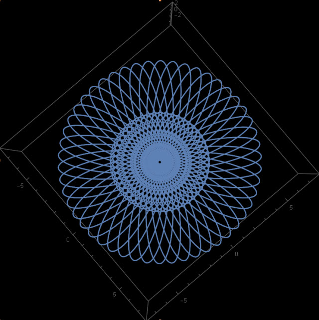
 That way we will obtain a trajectory. The axes of the tilted top will never coincide with the axes of the laboratory frame. Therefore the stereographically projected trajectory will never escape to infinity. We can plot it all. But one trajectory would be boring. It is better to tilt the laboratory frame (all the time by 30 degrees) using 50 different tilting axes (all in the xy plane. The following picture is then produced:
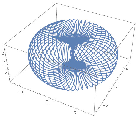

 the doubled kinetic energy is
  the parameter
  that we were using in the previous notes is
  The parameter
  is just zero,
  In what follows for simplicity we will take
 using stereographic projection described in
  by an angle
  can be described by (see Eq. (4) in
  matrix:
 in the formula!
 Then
Then  Therefore


 from
from  to
to 
 we have
  That is OK, because at
  we get
  That is the point representing the matrix
  It also describes the identity rotation in
  We get a straight path, the positive part of the z-axis. It is like the road in Nebraska at the top.