When we travel by a car, we decide which path to take. Choosing the right path may be crucial. Sometimes we choose a path that is straight, but nevertheless is scary. Like this road in Nebraska:

Sometimes the path is just “unusual”:

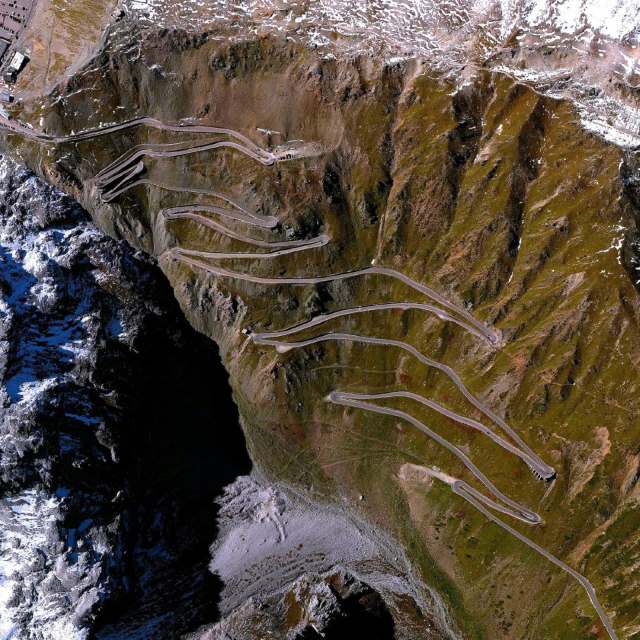
And sometimes we will think twice before choosing it:
We are interested in a particular kind of traveling: we want to travel in the rotation group. Think of an airplane. When it flies, it of course moves from a location to a location. But that is not what is of interest for us now. During the flight the plane turns and tilts, and all its turns and tilts can be (and often are) recorded. There are essentially three parameters that need to be recorded:
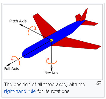
Usually they are referred to as roll, pitch and yaw. When you throw a stone in the air, and if you endow it with three axes, its roll, pitch, and yaw will also change with time. As there are three parameters, they can be represented by a point moving in a three-dimensional space. Instead of roll, pitch and yaw we could choose Euler angles. But, in fact, we will choose still another way of representing a history of tilts and turns of a rigid object as a path. We will use stereographic projection from the 3-dimensional sphere to the 3-dimensional Euclidean space.
You may ask: why to do it? What is the point? What can we learn from it? And my answer is: for fun.
One can also ask: what is the point with inspecting your hand? And yet there is the whole art of chiromancy, or palmistry. From Wikipedia:
Chiromancy consists of the practice of evaluating a person’s character or future life by “reading” the palm of that person’s hand. Various “lines” (“heart line”, “life line”, etc.) and “mounts” (or bumps) (chirognomy) purportedly suggest interpretations by their relative sizes, qualities, and intersections. In some traditions, readers also examine characteristics of the fingers, fingernails, fingerprints, and palmar skin patterns (dermatoglyphics), skin texture and color, shape of the palm, and flexibility of the hand.

We are going to learn about the lines in the rotation group. Some will be short, some will be long. We will learn how read from them about the body that recorded these lines during its flight.
From the internet we can learn:
Which Hand to Read
Before reading your palm, you should choose the right hand to read. There are different schools of thought on this matter. Some people think the right for female and left for male. As a matter of fact, both of your hands play great importance in hand reading. But one is dominant and the other is passive. The left hand usually represents what you were born with physically and materially and the right hand represents what you become after grown up. So, the right hand is dominant in palm reading and the left for supplement.
The same is with rotation groups. Which one to choose? We have rotations represented naturally as  orthogonal matrices, but we can also represent rotations by quaternions or by unitary matrices from the group
  Both play a great importance. We will choose unit quaternions or, equivalently,
  they seem to be primary!
Let us recall from Putting a spin on mistakes that every  unitary matrix
  of determinant one is necessarily of the form
(1) 
and it determines the rotation matrix 
(2) 
where  are real numbers representing a point on the three-dimensional unit sphere
  in the 4-dimenional Euclidean space
  that is
(3) 
The three-sphere is “homogeneous”, the same as the well-known two-sphere, like a table tennis ball.

And yet I want to paint one particular point on our three-sphere, namely the point represented by numbers  It follows from Eq. (2) that the rotation matrix corresponding to this particular point is the identity matrix:
![\[I=\begin{bmatrix}1&0&0\\0&1&0\\0&0&1\end{bmatrix}.\]](http://arkadiusz-jadczyk.eu/blog/wp-content/ql-cache/quicklatex.com-453acb12b4fd3acd05ad232ad4fd3158_l3.png "Rendered by QuickLaTeX.com")
I am not going to hide the fact that also the opposite point,  on our 3D ball also produces the identity rotation matrix, that is, in ordinary language: no rotation at all.
We are going now to go back to the stereographic projection that has been introduced already in Dzhanibekov effect – Part 2.
The idea is as in the picture below:

except that our sphere is 3-dimensional, and our plane onto which we are projecting is also 3-dimensional. Our North Pole is now the point  our South Pole the point and our “equator”, that is the set of all points on for which
  is now a 2-sphere rather than a circle like on the picture above. The projection formulas read (see Dzhanibekov effect – Part 2):
(4) 
The inverse transformation is given by
(5) 
where 
All the southern hemisphere (points on with  are projected inside the unit ball in
  ! The “equator”, where the three-sphere intersects the three-plane, is projected onto the unit sphere in
  The North Pole has no image, it is the only point on that has no image. In fact, it has an image, but at “infinity”. We will not need it. The South Pole, which, as we know, represents the trivial rotation, is mapped into the origin of , the point with
We will continue this course of rotational palmistry in the next posts.

 of complex
  given by Eq. (1) in
  we associate Hermitian matrix
 as in Eq. (10) in the previous post. We have orthogonal transformation
  defined by
![\[(R\vec{v})\cdot\vec{s}=U(\vec{v}\cdot\vec{s})\,U^*.\]](http://arkadiusz-jadczyk.eu/blog/wp-content/ql-cache/quicklatex.com-85f18b845d8f87bdcc01164b3cb8cb9d_l3.png "Rendered by QuickLaTeX.com")
 and that is where we left in the last note.
 We know (see the previous post) that
 It is now a straightforward calculation to express
  and
and  . But the calculation is long, and it is easy to make a mistake. That is why I used

 that maps
  that is every orthogonal matrix of determinant 1, is a rotation about some axis by some angle (and it is true). That is we can represent
 ![\[ R=\exp(\theta W(\vec{k})),\]](http://arkadiusz-jadczyk.eu/blog/wp-content/ql-cache/quicklatex.com-8783c14ce0f1cceb012228269e29984e_l3.png "Rendered by QuickLaTeX.com")
 is a unit vector. That was discussed in the note
  and then
  It is then the question of a straightforward calculation to verify that we get our

 . They are kinda OK, but they are not quite fitting our purpose. Therefore I will replace them with another set of matrices, and I will call these matrices
  They are defined the same way as Pauli matrices, except that
  has a different sign:


 would have in Eq. (
 satisfying:


 we would have to use
  in the above equations – which is not so nice. You would have asked: why minus rather than plus?
 – the first unit quaternion, from the imaginary complex number
  One should also note that the squares of the three imaginary quaternionic units, in their matrix realization, are
  that is “minus identity matrix”, instead of just number
  as in Hamilton’s definition.
 denotes Hermitian conjugation.
 is a sum:
![\[q= W+X\mathbf{i}+Y\mathbf{j}+Z\mathbf{k}.\]](http://arkadiusz-jadczyk.eu/blog/wp-content/ql-cache/quicklatex.com-2a664d71a7504a771bc2740d015508b4_l3.png "Rendered by QuickLaTeX.com")

 is represented by Hermitian conjugated matrix. Notice that
  Unit quaternions are quaternions that have the property that
  They are represented by matrices
  such that
  that is by unitary matrices. Moreover we can check that then
![\[\det Q=\det \begin{bmatrix}W+iZ&iX-Y\\iX+Y&W-iZ}\end{bmatrix}=W^2+X^2+Y^2+Z^2=1.\]](http://arkadiusz-jadczyk.eu/blog/wp-content/ql-cache/quicklatex.com-f7194bb3c88ae0249fef9a8eae5320f9_l3.png "Rendered by QuickLaTeX.com")
![\[ U=\begin{bmatrix}a&b\\c&d\end{bmatrix}.\]](http://arkadiusz-jadczyk.eu/blog/wp-content/ql-cache/quicklatex.com-7928d1bdffa0b81bd1fc0bfde23dbc03_l3.png "Rendered by QuickLaTeX.com")
 we can easily check that
![\[\begin{bmatrix}a&b\\c&d\end{bmatrix} \begin{bmatrix}d&-b\\-c&a\end{bmatrix}=I.\]](http://arkadiusz-jadczyk.eu/blog/wp-content/ql-cache/quicklatex.com-b009fb19f11d5183b37960d05f03672d_l3.png "Rendered by QuickLaTeX.com")
![\[ U^{-1}=\begin{bmatrix}d&-b\\-c&a\end{bmatrix}.\]](http://arkadiusz-jadczyk.eu/blog/wp-content/ql-cache/quicklatex.com-da4c69e1a390cf0c0869556445ad4591_l3.png "Rendered by QuickLaTeX.com")
 But
But ![\[ U^*=\begin{bmatrix}\bar{a}&\bar{c}\\\bar{b}&\bar{d}\end{bmatrix}.\]](http://arkadiusz-jadczyk.eu/blog/wp-content/ql-cache/quicklatex.com-e058e0b1d973efa2de694f8e73b30ee1_l3.png "Rendered by QuickLaTeX.com")
![\[\begin{bmatrix}d&-b\\-c&a\end{bmatrix}=\begin{bmatrix}\bar{a}&\bar{c}\\\bar{b}&\bar{d}\end{bmatrix}.\]](http://arkadiusz-jadczyk.eu/blog/wp-content/ql-cache/quicklatex.com-07c4fac56c58a7b776693fc2b3533b80_l3.png "Rendered by QuickLaTeX.com")
 Writing
  we get the form (
 and
and  operators), but that was pretty soon abandoned. Mathematicians at that time were complaining that
  in our 3D space we can associate Hermitian matrix
  of trace zero:

![\[ \vec{v}\cdot\vec{s}\mapsto U\vec{v}\cdot\vec{s}\, U^*.\]](http://arkadiusz-jadczyk.eu/blog/wp-content/ql-cache/quicklatex.com-1940556b785f9b3ddc697de6bcd7afe0_l3.png "Rendered by QuickLaTeX.com")
 is also Hermitian. Since
  such that:
![\[\tilde{ \vec{v}}\cdot\vec{s}=U\vec{v}\cdot\vec{s}\,U^*.\]](http://arkadiusz-jadczyk.eu/blog/wp-content/ql-cache/quicklatex.com-9885c1977876d2b54af4bf176127ed7a_l3.png "Rendered by QuickLaTeX.com")
 , then
  Therefore we must have
  In other words the transformation (which is linear)
  is an isometry – it preserves the length of all vectors. And it is known that every isometry (that maps
  into
into  This way we have a map from
  – the group of orthogonal matrices. We do not know yet if
  which is the case, but it needs a proof, some proof….


