We start with a partial recall of events as they transpired so far. A month ago we became hyperbolic. The post Getting hyperbolic started with this sentence:
Without knowing it, during the last three posts (Our first field expedition, Our second field expedition, The Third Expedition) we became hyperbolic. Hyperbolic and conformal. Conformal and relativistic, relativistic and non-Euclidean.
Then we introduced the group SU(1,1) and its action on the disk. Then, in From SU(1,1) to the Lorentz group we realized that the disk can be considered as a projection of a hyperboloid in 2+1 dimensional space-time, where the hyperboloid is inside the future light cone. We were contemplating the image below

and we have shown that there is a group homomorphism from SU(1,1) to the Lorentz group SO(2,1) of 2+1 dimensional special relativity. We have calculated the formula explicitly in Eq. (7) there. If ![A=\left[\begin{smallmatrix}\lambda&\mu\\ \bar{\mu}&\bar{\lambda}\end{smallmatrix}\right]](http://arkadiusz-jadczyk.eu/blog/wp-content/ql-cache/quicklatex.com-2e511c5cae985c3970df6ef6d1883bab_l3.png "Rendered by QuickLaTeX.com") is a complex matrix from SU(1,1) with
is a complex matrix from SU(1,1) with  split into real and imaginary parts, then the real
  matrix
  from SO(2,1) is given by the formula:
(1) 
The map  is a group homomorphism, that is
  and
and  ( Of course in we denote by the same symbol
  identity matrices of different sizes.)
After that, in Getting real, we used Cayley transform that defines group isomorphism between the complex matrix group SU(1,1) and the real matrix group SL(2,R). With
(2) 
(3) 
we have that if ![A'=\left[\begin{smallmatrix}\alpha&\beta\\ \gamma&\delta\end{smallmatrix}\right]](http://arkadiusz-jadczyk.eu/blog/wp-content/ql-cache/quicklatex.com-8969b960a5764336f49fd61d00bb538d_l3.png "Rendered by QuickLaTeX.com") is a real matrix from SL(2,R) (i.e.
is a real matrix from SL(2,R) (i.e.  ), then
  is in SU(1,1). If we calculate explicitly
  and
and  in terms of
  the result is:
(4) 
Combining it with we obtain group homomorphism from SL(2,R) to SO(2,1). Explicitly
(5) 
So far, so good, but now there comes real magic!

We do not have to travel around the world, through SU(1,1) and hyperboloids. We will derive the last formula directly using a method that is similar to the one we used when deriving the map from quaternions to rotation matrices in Putting a spin on mistakes.
The Lie algebra sl(2,R) of the Lie group SL(2,R) consists of real  matrices of zero trace – we call them “generators”. We already met three particular generators
  , for instance in SL(2,R) generators and vector fields on the half-plane, and I will skip this time primes as they have been denoted previously
(6) 
Every element of sl(2,R) is a real linear combination of these three. So, can be considered as a basis of sl(2,R). For instance in SL(2,R) generators and vector fields on the half-plane we constructed a particular generator  and
and  defined as
(7) 
The Lie algebra sl(2,R) is a three-dimensional real vector space. But it is more than just a vector space. The group SL(2,R) acts on this space by what is called “the adjoint representation”. This is true for the Lie algebra of any Lie group. Here we have a particular case. Namely, if  is in sl(2,R), that is if has trace zero, and if
  is in SL(2,R), that is the determinant of is one, then
  is also of zero trace (we do not need the property of determinant one for this). The map
  is a linear map. Thus we have action, let us call it
  , of SL(2,R) on sl(2,R):
(8) 
Remark: I will now be skipping primes that I was using to distinguish matrices from SL(2,R) from matrices from SU(1,1).
Evidently (from associativity of matrix multiplication) we have
![\[\mathcal{L}(A_1A_2)=\mathcal{L}(A_1)\mathcal{L}(A_2).\]](http://arkadiusz-jadczyk.eu/blog/wp-content/ql-cache/quicklatex.com-eaf44c72fe09ddc3fb2e0378a0344943_l3.png "Rendered by QuickLaTeX.com")
Usually instead of  one writes
  and uses the term “adjoint representation”. In short: the group acts on its Lie algebra by similarity transformations. Similarity transformation of a generator is another generators. Even more, by expanding exponential into power series we can easily find that
(9) 
So sl(2,R) is a three dimensional real vector space and SL(2,R) acts on it by linear transformations.
But that is not all. In sl(2,R) we can define a very nice scalar product  as follows
(10) 
where  is the trace of the product of matrices and
Why is this scalar product “nice”? What is so nice about it? It is nice, because with this scalar product the transformations are all isometries – they preserve this scalar product:
(11) 
The derivation of this last property follows from the definitions and from the property that similarity transformations do not change the trace.
So sl(2,R) is a three dimensional real vector space with a scalar product. But in sl(2,R) we have our basis  It is easy to calculate scalar products of the basis vectors. We get the following matrix for the matrix
  with entries
(12) 
(13) 
Thus sl(2,R) has all the properties of the Minkowski space with two space and one time dimensions. The generator  has “time direction”, while
  are “space directions”.
Once we have a basis there, we can calculate the components of the transformations in this basis:
(14) 
I used Mathematica to calculate  for
for ![A=\left[\begin{smallmatrix}\alpha&\beta\\ \gamma&\delta\end{smallmatrix}\right]](http://arkadiusz-jadczyk.eu/blog/wp-content/ql-cache/quicklatex.com-969779c63def79263f77beb857467082_l3.png "Rendered by QuickLaTeX.com") . Here is the result:
. Here is the result:
(15) 
Here I admit that in this last formula I did copy and paste from Eq. (5) above. Because indeed that is what happened in the calculation – the result came identical. And that is the real magic. We do not need external space-time and hyperboloids. Everything is already contained in the group itself and in its Lie algebra!
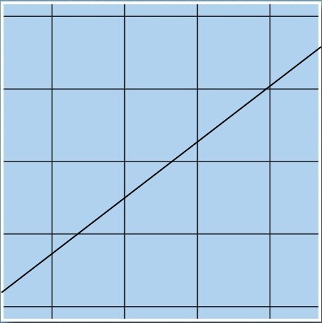
 is a vertical line, then
  therefore
  In
In 


 and
and  on the vertical line must be proportional:
 is an “affine parameter”: it is proportional to the arc length, possibly translated. In fact that is part of the definition of the geodesic that enters the “Noether’s theorem” that we are using. Usually we choose the proportionality constant equal to one.
 Choosing the constant equal to 1, we have

 is of unit length. In our case that is equivalent to
 or
or  or
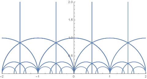
or  , so that there are three kinds of geodesics. In physics this happens for space-time metrics with Minkowski signature, and in multi-dimensional Kaluza-Klein theories. We will discuss another such case in the following posts.
 is some function of the arc length parameter
  , and substitute into Eqs. (


 has components

 is obtained by taking derivatives with respect to

 on our line:
 here:
here:
 Its scalar products with
  and
and  should be constant. But now we remember that in calculating the scalar product we must use Eq. (


 on
on  -axis and radius
  has equation:
 and differentiating with respect to


