According to Wikipedia
In differential geometry, a geodesic is a generalization of the notion of a “straight line” to “curved spaces”.
…
The first line in the online Encyclopedia of mathematics is similar
The notion of a geodesic line (also: geodesic) is a geometric concept which is a generalization of the concept of a straight line (or a segment of a straight line) in Euclidean geometry to spaces of a more general type.
…
Wolfram’s MathWorld is somewhat more original:
A geodesic is a locally length-minimizing curve. Equivalently, it is a path that a particle which is not accelerating would follow. In the plane, the geodesics are straight lines. On the sphere, the geodesics are great circles (like the equator). The geodesics in a space depend on the Riemannian metric, which affects the notions of distance and acceleration.
…
It is time for us to study geodesics on the upper half-plane, and do it in a semi-rigorous way. That would require a rigorous definition of geodesics, which would take us into differential geometry and variational calculus. That would certainly not be a length-minimizing and straight way of achieving our goal. For us, interested mainly in Lie groups and their actions, there is a shorter way. It is like in classical mechanics, where in many important cases we do not have to solve complicated Newton’s differential equations, it is enough to use the law of conservation of energy, or momentum.
That is what we will do. We will use conservation laws. Usually these come as theorems in courses of differential geometry (Noether’s theorem). For instance Sean Carroll in his online book Lecture Notes on General Relativity, in Chpater 5, More geometry has this piece:
And that is what we will use. And how to use it, in detail, we will see below.
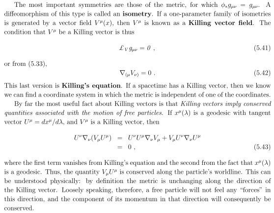
Let us start with this sentence:
If a one-parameter family of isometries is generated by a vector field
, then
is known as a Killing vector field.
We have our candidates for Killing vector fields. We were plotting some of their streamlines in SL(2,R) generators and vector fields on the half-plane .
But are we sure that they generate “isometries”? Till now we have only a roundabout argument: metric on the upper half-plane comes from the metric on the disk, metric on the disk comes from geometry on the hyperboloid, metric on the hyperboloid comes from flat space-time metric of signature  and the SL(2,R) group comes from the SO(2,1) group of linear transformations preserving the flat space-time metric. That could be enough for a while, but can’t we check directly if indeed we have isometries?
Yes, we can check, and that is, in fact, quite easy. Generators of the SL(2,R) group form the Lie algebra sl(2,R) of real  matrices of trace zero. After exponentiation they generate one-parameter groups of SL(2,R) matrices. SL(2,R) acts on the upper-half plane
  by linear fractional transformations. If
  is in SL(2,R)
(1) 
 then
then (2) 
Is the transformation defined in Eq. (2) an isometry? The formula looks relatively simple when written in terms of complex variables. But if we write  then the coordinates
  of the transformed point become not that simple functions of the coordinates
  of the original point:
(3) 
(4) 
Is it an isometry? And what is isometry?
In Conformally Euclidean geometry of the upper half-plane we have derived the formula for calculating the length of a given curve:
(5) 
Now, suppose, we transform our curve using the matrix . The length of the transformed curve is then given by the formula
(6) 
where the relation between and is given by Eqs. (3,4).
The transformation is an isometry if  for any segment of any curve. Is true in our case? In order to verify it some little calculations are needed. If we listen to Leibniz:

— Gottfried Leibniz
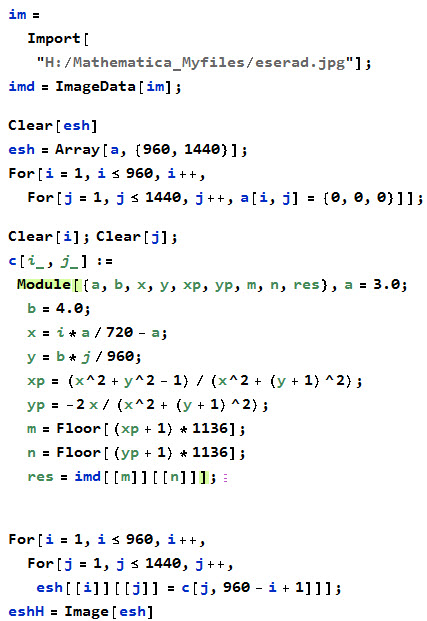
we use our computer. I used Mathematica. Here is the result:

To summarize: after somewhat lengthy calculation we end up with
(7) 
even without using the  condition. Therefore SL(2,R) transformations are indeed isometries (for our metric). Therefore our vector fields are “Killing vector fields”. Therefore we can use their properties in our derivation of geodesic equations. Which we will continue in the following post.

 is a parametric equation of the curve, then
  and so

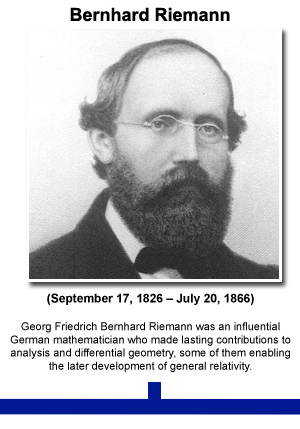
 . Development of Riemannian geometry resulted in synthesis of diverse results concerning the geometry of surfaces and the behavior of geodesics on them, with techniques that can be applied to the study of differentiable manifolds of higher dimensions.
![\[ds^2=\begin{bmatrix}dx&dy\end{bmatrix}\begin{bmatrix}g_{xx}&g_{xy}\\g_{yx}&g_{yy}\end{bmatrix}\begin{bmatrix}dx\\dy\end{bmatrix}= g_{xx}dx^2+2g_{xy}dx\,dy+g_{yy}dy^2,\]](http://arkadiusz-jadczyk.eu/blog/wp-content/ql-cache/quicklatex.com-942c3a90f1220596b77d711e33ad5d35_l3.png "Rendered by QuickLaTeX.com")
 ) “Riemannian metric” matrix
![\[g=\begin{bmatrix}g_{xx}&g_{xy}\\g_{yx}&g_{yy}\end{bmatrix}.\]](http://arkadiusz-jadczyk.eu/blog/wp-content/ql-cache/quicklatex.com-aed021f610b4c8dc841e7b55ad71977a_l3.png "Rendered by QuickLaTeX.com")

 and
and  . Or
. Or
 and
and  are two tangent vectors at
  then their scalar product is given by a general formula

 are two tangent vectors at
  then the angle
  between them is defined through the formula:
 and
and  are their norms. If we use the scalar product given by Eq. (
 in
in  cancels out with the product of denominators is the norms. The end result is

 that differ a scalar factor
  we say that they are conformally related, or conformal to each other. In our case the metric
  These two symmetries are horizontal translation and uniform dilation. The horizontal translational symmetry means that all geometric properties of objects are invariant when all parts of the object keep the same height (constant
  ), and only the
  coordinate is translated by a fixed amount. The symmetry with respect dilations means that when we multiply all


 and
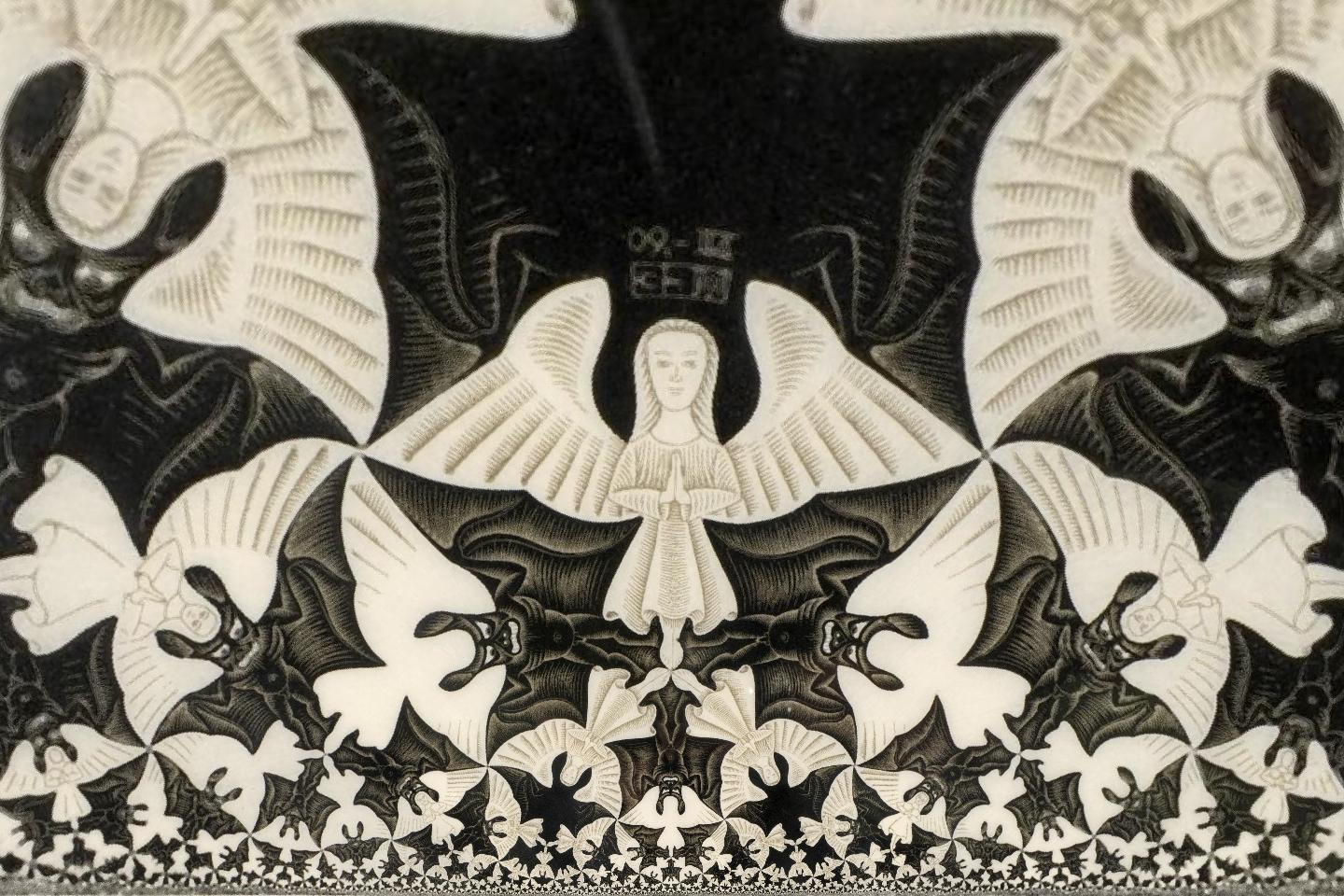
and  The part of the disk that is not being used is then small enough not to worry about (on the right in the image, near
  on the circle boundary ). That gives the ratio 3:2 of the image. I decided to create 1440×960 pixels image. For this I had to find on the net Esher’s Limit Circle with high enough resolution. I have found it