Comments on Clifford algebras

In November 2015 I was reading “Quantum mechanics and gravity” by Mendel Sachs [1]. There, on p. 46 I have found the following piece that got my interest

We may exploit these ideas of generalizing Einstein’s tensor formalism by starting with the invariant differential metric in a Riemannian spacetime:

(3.10)   \[ds = q^\mu(x)dx_\mu,\]

where q^\mu is a four-vector field (dependent on all of the coordinates x of spacetime) in which all four vector components are quaternion-valued, rather than being real-number valued. Thus the generalized metrical field q^\mu is a 16-component variable. The invariant metric ds of (3.1) is a factorization of the Riemannian metric,

(3.2)   \[ds^2=g^{\mu\nu}dx_\mu dx_\nu = ds \,ds^*.\]

where the asterisk denotes the quaternion conjugate of ds (corresponding to time reversal or space reflection).

The correspondence between the metric tensor and the quaternion metric is then, from (3.1) and (.2),

    \[g^{\mu\nu}\Leftrightarrow -\frac{1}{2}(q^\mu q^{*\nu}+q\nu q^{*\mu}),\tg{3.3}\]

where the minus sign is chosen because of normalization.

Sachs goes then on to derive “quaternion field equations”. I got interested. After some search I have found the 1968 paper by H. G. Loos [2] criticizing Sachs’ idea of “factorizabiility of Einstein’s equations”, together with Sachs’ reply [3].

I looked and it was rather clear to me that Loos was right, nevertheless Sachs evidently persisted till 2004, and Springer did not do too well with their peer review. For some reason they were suspiciously forgiving.

Anyway I got interested and it was clear to me that Sachs used quaternions where Clifford algebras were more appropriate. Probably he did not know much about them and quaternions sounded like something more mysterious. So I decided to come back to my studies of Clifford algebras. I have used them before in my papers on conformal compactification of the Minkowski space and also in my book about Quantum Fractals. But this time I decided to study also more general Clifford algebras, namely those corresponding to possibly degenerate metrics. In fact at some point in the past I got interested in degenerate metric and wrote a paper on this subject [6] – though never published in a journal. Recently while reading “warped Passages” by Lisa Randall [7] it occured to me that Clifford algebras with degenerate metric may find new applications in multidimensional models, wher our four dimensional space time is embedded as a singular brane in a higher dimensional geometry. Sub-Riemannian geometry that I was always neglecting ay be of help here.

So I got again interested in Clifford algebras, but this time paying attention also to those features that survive when the metric becomes degenerate. In fact the exterior algebra is a special case of the Clifford algebra, therefore whoever is interested in multivectors must also be interested in Clifford algebras with degenerate metric. Physicists, till now, are either using exterior algebra, which means Clifford algebra for zero metric, or “space-time algebra” which is Clifford algebra with (nondegenerate) Minkovski metric. But what happens in between? What kind of mathematics is there?

Very soon I discovered that the subject has been discussed in the literature, mainly by Ablamowicz [8] and Ablamowicz and Lounesto [9]. It has even morphed into the discussion of “Clifford algebras of a bilinear form with an antisymmetric part” [10]. But then I noticed that these authors are quoting 1986 paper by Oziewicz [11], but they are not quoting the classic Bourbaki 1959 [12]. It appeared to me that this particular part of the Bourbaki’s “Elements of Mathematics”, dealing with sesquilinear and quadratic forms, has not been translated from French into English. If that is true, then I do not understand why? It is a beautiful exposition of the theory of quadratic forms and Clifford algebras, and evidently not always taking the same path as the treatice by Chevalley, even if Chevalley was a member of the Bourbaki group.

I started to study Bourbaki’s Algebra Chapter 9 and realized that it contains real pearls – it contains results and formulas that later on have been “discovered” and popularized among physicists by Oziewicz, Hestenes, Graf, Lounesto, Ablamowicz , and that applies as well to the case of nondegenerate quadratic forms!

At that point I decided to start writing my own “Notes on Clifford Algebras” – which is my own rewriting of what I have found in Bourbaki and elsewhere, together with step-by-step expanding the subject, adding observations that I consider as interesting.

My Notes on Clifford Algebras are available at this link.

At present, and I am writing this post on January 24, 2019, there are 22 pages, and it is release version 0.8b. Every couple of days I am adding something new or improving. Therefore I will continue this post adding “What’s new” with each version update.
References
[1] Mendel Sachs, Quantum Mechanics and Gravity, Springer 2004
[2] H. G. Loos, Factorizability of Einstein’s Field Equations, Nuovo Cimento, 55 B, 339-343, 1968
[3] M. Sachs, Comments on a letter by H. G. Loos on “Factorizability of Einstein’s Field Equations”, Lett. Nuovo Cimento, vol. 1 N 15, 741-745, 1969
[4] A. Jadczyk, On Conformal Infinity and Compactifications of the Minkowski Space, Advances in Applied Clifford Algebras, 21 N 4, 721-756, 2011
[5] A. Jadczyk, Quantum Fractals, World Scientific 2014
[6] A. Jadczyk, Vanishing Vierbein in Gauge Theories of Gravitation, arXiv:gr-qc/9909060v1
[7] Lisa Randall, Warped Passages, HarperCollins 2006
[8] Rafal Ablamowicz, Structure of spin groups associated with degenerate Clifford algebras, Journal of Mathematical Physics, 27, 1-6, 1986
[9] Rafal Ablamowicz and Pertti Lounesto, Primitive Idempotents and Indecomposable Left Ideals in Degenerate Clifford Algebras, in J. S. R. Chisholm and A. K. Common ed, Clifford Algebras and Their Applications in Mathematical Physics, Reidel 1986
[10] Rafal Ablamowicz and Pertti Lounesto, On Clifford Algebras of a Bilinear Form with an Antisymmetric Part, in R. Ablamowicz and J. M. Parra and P. Lounesto ed., Clifford Algebras with Numeric and Symbolic Computations, Birkhäuser 1966
[11] Zbigniew Oziewicz, From Grassmann to Clifford, in Clifford Algebras and Their Applications in Mathematical Physics, 1986, op. cited
[12] N. Bourbaki, Algèbre – Chapitre 9. Hermann, 1959.
[13] Claude Chevalley, The Algebraic Theory of Spinors and Clifford Algebras: Collected Works, Volume 2, Springer 1996.

What’s new v0.8c, 26/1/2019

Added 1.1.5 Diagonalization of symmetric bilinear forms
Added Even and odd subalgebras at the end of 1.2.2 Main involution and main anti-involution
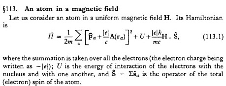
Comment on “Could ordinary quantum mechanics be just fine for all practical purposes?” by Alexey Nikulov

Abstract: Contrary to the claim by Alexey Nikulov it is argued that there is no error in Landau and Lifshitz derivation of magnetic coupling formula (113.2)

In [1], Sec. 4.3, “Quantum mechanics cannot describe both opposite cases”, Alexey Nikulov claims that Landau and Lifshitz have made an error deriving, in their quantum theory textbook [2], the formula for the coupling of the angular momentum to the magnetic field in their chapter on “An atom in a magnetic field”. More specifically Nikulov claims in [1] that the formula (113.2) in [2] is obtained by Landau and Lifshitz from (113.1) by an “illegal substitution” or, by an “elementary arithmetic error” [3].

While it is true that Landau and Lifshitz could have been more explicit in their derivation, I will derive their (113.2) from (113.1) in all detail – showing that their is no “arithmetic error”, and that it is, in fact, Alexey Nikulov who made an error misunderstanding the arguments in Ref.[2] and “overshooting” with his criticism.

As it is very important to pay attention to details, let us start with an exact image (see Fig. 1) of the starting formula (113.1) in Ref. [2]:

Fig. 1. Landau-Lifshitz p.461, Eq. (113.1)

A. Nikulov is questioning the derivation, given in Ref. [2], of the following formula copied here from Ref. [2] in Fig. 2 below.


Fig. 2, Landau-Lifshitz p.461, Eq. (113.2)

The Bohr magneto \mu_B is defined here as \mu_B=|e|\hbar/2mc. We will neglect spin \hat{\mathbf{S}} and the scalar potential U, and write down the the starting formula just for one electron, setting c=1:

Remark: These simplifying assumptions can be made without losing the essence of the argument.

Thus our starting formula, which we denote as ((113.1)) reads as follows

((113.1))   \begin{equation*} \hat{H}=\frac{1}{2m}\left(\hat{\mathbf{p}}+|e|\mathbf{A}\right)^2,\end{equation*}

where

(1)   \begin{equation*} \hat{\mathbf{p}}=-i\hbar \nabla\end{equation*}

is the canonical momentum vector operator and \mathbf{A} is the vector potential for the magnetic field \mathbf{H}:

(2)   \begin{equation*} \mathbf{H}=\nabla\times\mathbf{A}.\end{equation*}

The electron charge (negative) is e=-|e|.

In order to derive the formula (113.2) of Ref. [2] we need to calculate the Hamiltonian \hat{H} explicitly. To this end we take the square:

(3)   \begin{eqnarray*} \hat{H}&=&\frac{1}{2m}\left(\hat{\mathbf{p}}+|e|\mathbf{A}\right)^2\nonumber\\ &=&\frac{1}{2m}\hat{\mathbf{p}}^2+\frac{ |e|}{2m}\hat{\mathbf{p}}\cdot \mathbf{A}+\frac{|e|}{2m}\mathbf{A}\cdot \hat{\mathbf{p}}+\frac{|e|^2}{2m}\mathbf{A}^2.\end{eqnarray*}

Following Ref. [2] we introduce \hat{H}_0 defined as

(4)   \begin{equation*} \hat{H}_0=\frac{1}{2m}\hat{\mathbf{p}}^2,\end{equation*}

where \hat{\mathbf{p}} is the canonical momentum defined in Eq. (1).
Then, using Eq. (4) we can rewrite (3) as

(5)   \begin{equation*} \hat{H}=\hat{H}_0+\frac{ |e|}{2m}(\hat{\mathbf{p}}\cdot \mathbf{A}+\mathbf{A}\cdot \hat{\mathbf{p}})+\frac{|e|^2}{2m}\mathbf{A}^2.\end{equation*}

The vector potential \mathbf{A} is a function of coordinates, therefore in general it will not commute with the components of the canonical momentum operator. We have

(6)   \begin{equation*} \hat{\mathbf{p}}\cdot \mathbf{A}=\mathbf{A}\cdot\hat{\mathbf{p}}-i\hbar \nabla\cdot\mathbf{A}.\end{equation*}

We consider the case of a uniform magnetic field, i.e. the vector \mathbf{H} is constant. Then \mathbf{A} can be chosen as

((111.7))   \begin{equation*} \mathbf{A}=\frac{1}{2}\mathbf{H}\times\mathbf{r}.\end{equation*}

In this case, with \mathbf{A} given by ((111.7)) we have \nabla\cdot \mathbf{A}=0,
therefore \mathbf{p}\cdot\mathbf{A}=\mathbf{A}\cdot \mathbf{p}. Thus \hat{H}, given by Eq. (3), takes the form:

(7)   \begin{equation*} \hat{H}=\hat{H}_0+\frac{ |e|}{m}\mathbf{A}\cdot \hat{\mathbf{p}}+\frac{|e|^2}{2m}\mathbf{A}^2,\end{equation*}

or, making use of Eq. ((111.7)) again:

(8)   \begin{equation*} \hat{H}=\hat{H}_0+\frac{ |e|}{2m}(\mathbf{H}\times\mathbf{r})\cdot \hat{\mathbf{p}}+\frac{e^2}{8m}\,(\mathbf{H}\times\mathbf{r})^2.\end{equation*}

Using the standard vector product identity

(9)   \begin{equation*} (\mathbf{H}\times\mathbf{r})\cdot \hat{\mathbf{p}}=\mathbf{H}\cdot (\mathbf{r}\times\hat{\mathbf{p}})\end{equation*}

we can rewrite the second term to obtain

(10)   \begin{equation*} \hat{H}=\hat{H}_0+\frac{ |e|}{2m}\mathbf{H} \cdot (\mathbf{r} \times \hat{\mathbf{p}})+\frac{e^2}{8m}\,(\mathbf{H}\times\mathbf{r})^2.\end{equation*}

We now introduce canonical angular momentum operator \hat{\mathbf{L}} defined as

(11)   \begin{equation*} \hat{\mathbf{L}}=\mathbf{r}\times\hat{\mathbf{p}}.\end{equation*}

Then

(12)   \begin{equation*} \hat{H}=\hat{H}_0+\frac{ |e|}{2m}\mathbf{H} \cdot \hat{\mathbf{L}}+\frac{e^2}{8m}\,(\mathbf{H}\times\mathbf{r})^2.\end{equation*}

The above is Eq. (113.2) of Ref. \cite{LandauL} that we have derived step by step, and without any “arithmetic errors”. Therefore the part of Ref. \cite{nikulov2016} questioning the validity of this derivation is erroneous.

It is nevertheless interesting to try to understand why such an wrong conclusion could arise. The following is my guess based on the following sentence in Sec. 4.3 of Ref. [1]:
\begin{quotation}“The additional summand \mu_B\hat{L}B could appear in the relation (113.2) due to illegal substitution of P^2/ 2m by m\hat{v}^2/2 in \hat{H}_0.”\end{quotation}

While in quantum mechanics we do have the canonical momentum operator (see Eq. (1), there is no canonical velocity operator. The explicit expression for the velocity operator must be calculated for each Hamiltonian separately. Given a Hamiltonian \hat{H} (assuming not time dependent) the corresponding velocity operator is defined by

(13)   \begin{equation*} \hat{\mathbf{v}}=\frac{i}{\hbar}[\hat{H},\mathbf{r}].\end{equation*}

Its expectation value \langle \bv\rangle|_{\psi(t)} is equal to the time derivative of the expectation value of the position operator.

For a free particle, when \hat{H}=\hat{H}_0=\frac{\hat{p}^2}{2m}, we find that
the expression for the velocity operators is given by

(14)   \begin{equation*} \hat{\mathbf{v}}=\frac{i}{\hbar}[\hat{H_0},\mathbf{r}]=\frac{\mathbf{p}}{m}.\end{equation*}

For a particle in a magnetic field \mathbf{H}=\nabla \times \mathbf{A} the Hamiltonian \hat{H} is defined by Eq. ((113.1)), that is:

(15)   \begin{equation*} \hat{H}=\frac{\hat{\pi}^2}{2m}, \end{equation*}

where the kinetic momentum \hat{\boldsymbol{\pi}} is defined as

(16)   \begin{equation*} \hat{\boldsymbol{\pi}}=\hat{\mathbf{p}}-e\mathbf{A}.\end{equation*}

In this case the velocity operator \hat{\mathbf{v}} is given by a different expression than that in the free case:

(17)   \begin{equation*} \hat{\mathbf{v}}=\frac{i}{\hbar}[\hat{H},\mathbf{r}]=\frac{\boldsymbol{\pi}}{m}.\end{equation*}

In both cases the Hamiltonian can be written as the kinetic energy m\hat{v}^2/2, but the expression in terms of the canonical momenta and positions is different in each case. Nikulov seems to claim that it is impossible to derive the second term in Eq. ((113.2)), the one containing the coupling of the magnetic field to the angular momentum, from “just the kinetic energy” because he fails to notice that the kinetic energy’ has a different expression for a particle in a magnetic field than the one without. It is for this reason that the whole section of Ref. [1] needs to be completely rewritten.
References
[1] Alexey Nikulov, Could ordinary quantum mechanics be just fine for all practical purposes?, Quantum Stud.: Math. Found. (2016) 3: 41., doi: 10.1007/s40509-015-0057-3 (see also arXiv:1508.03505)
[2] Landau, L. D., Lifshitz, E. M.: Quantum Mechanics: Non-Relativistic Theory. Volume 3, Third Edition, Elsevier Science, Oxford, 1977.
[3] Alexey Nikulov, private communication

Addendum 1:
On March 9, 2018 I receive en email from A. Nikulov containing the following statements:

В разложении бинома на слагаемые (p – qA)^2/2m = p^2/2m – pqA/m + (qA)^2/2m в книге LL принимается, что первое слагаемое описывает атом без магнитном поле, а два других в магнитном поле. Это не только нельзя ничем обосновать, но и приводит к очевидной арифметической ошибки.

Translating into English:

In the decomposition of the binom into separate terms (p – qA)^2/2m = p^2/2m – pqA/m + (qA)^2/2m in the LL book it is assumed that the first term describes the atom without the magnetic field, while two other in a magnetic field. Not only there is no way to justify it, but also it leads to an evident arithmetic error.

Again A. Nikulov is making an error. The first term is nothing else but \hat{H}_0, which is the same as \hat{H} with \mathbf{A} set to zero, that is the free Hamiltonian, corresponding to the atom without the magnetic field. It is not true that Landau and Lifshitz state that two other term describe the atom in a magnetic field. They do not say so. What describes the atom in magnetic field is all three terms. All that is evident and follows from the definitions. There is nothing that need to be justified and there are no arithmetic errors.

Addendum 2:

As a reply to the Addendum 1 above, I received the following:


я не понимаю, где я опять сделал ошибку. Я согласен с тем, что The first term is nothing else but Н_0, which is the same as Н with А set to zero, that is the free Hamiltonian, corresponding to the atom without the magnetic field. Но я не могу согласится с тем, что It is not true that Landau and Lifshitz state that two other term describe the atom in a magnetic field. Даже если Landau and Lifshitz об этом ничего не написали, то что two other term describe the atom in a magnetic field очевидно из того, А в них не равно нулю. Приравняйте в выражении (8) или (10) Вашего Comment магнитное поле нулю во всех слагаемых (а не в одном!) и Вы получите выражение Н = Н_0 без арифметической ошибки (в котором кинетическая энергия равняется кинетической энергии), но и без энергии магнитного момента в магнитном поле. Мне странно объяснять, что нельзя в одном слагаемом суммы принять А = 0, а в остальных оставить ненулевое значение А. Но мне пришлось это сделать в очередном комментарии к своей статье “Could ordinary quantum mechanics be just fine for all practical purposes?” на ResearchGate. Неужели Вам непонятно, если сделать такую же глупость, какая сделана в книге Landau and Lifshitz, то мы получим арифметическую ошибку?

Below is my English translation of the relevant part, separated into two parts, intertwined with my explanations.

I do not understand when have I made again an error. I agree that “The first term is nothing else but Н_0, which is the same as Н with А set to zero, that is the free Hamiltonian, corresponding to the atom without the magnetic field.” But I cannot agree that it is not true that “Landau and Lifshitz state that two other term describe the atom in a magnetic field. Even if Landau and Lifshitz did not write it, it is clear that the two other terms describe the atom in a magnetic field, because A there is not equal zero.

My comment: Because we are discussing questions of “arithmetic errors” and “illegal substitutions” in a popular textbook, it is very important to be very precise and logically impeccable. The way it stated in the quotation above it is not logically precise and it is potentially misleading. The two terms do not constitute the full description of the atom in a magnetic field. The full description is given by all three terms together. The first term is the kinetic energy of the free particle. The second term is the linear coupling of the angular momentum to the magnetic field, the third term, quadratic in the magnetic field, is usually neglected completely for weak magnetic fields.

Perhaps it should also be stated why sometimes the talk is about the atom, while only electron figures out in the Hamiltonian. The reason is that the terms are inversely proportional to the mass, therefore the proton energy terms are small compared to the electron energy terms and can be neglected.

If you set magnetic field to zero in the expression (8) or (10) of your comment in all terms, (and not only in one!) then you will get the expression H=H_0 without arithmetic error (in which kinetic energy is equal to the kinetic energy), but without the energy of the magnetic moment in magnetic field. t is strange that I have to explain that you should not to set A=0 in one term, and to let it to be non-zero elsewhere.

The sentence above does not make sense. In fact H_0 has been obtained from (8) or (10) by setting the magnetic field to zero in all terms.

Spinning Top – Space Odity

I start with quoting from Wikipedia:

Peggy Annette Whitson (born February 9, 1960) is an American biochemistry researcher, NASA astronaut, and former NASA Chief Astronaut. Her first space mission was in 2002, with an extended stay aboard the International Space Station as a member of Expedition 5. Her second mission launched October 10, 2007, as the first woman commander of the ISS with Expedition 16. She is currently in space on her third long-duration space flight and is the current commander of the International Space Station.

Two weeks ago we could see live how “Kimbrough and Flight Engineer Peggy Whitson of NASA reconnect cables and electrical connections on PMA-3 at its new home on top Harmony”

That is surely fascinating, but what we are particularly interested in the spinning top in zero gravity experiments on the board of ISS in 2013

At 0:42 in this video Peggy tells us that:

“Conservation of angular momentum keeps the top axis pointed in the same direction”

We look at it, and we compare with the other video featuring the Dzhanibekov effect

The same effect I have modeled with Mathematica:

is even better visible here:

There is also conservation of angular momentum there, but the axis of rotation evidently is not being kept all the time in the same direction. Once in while, quasi-periodically, it flips.

What’s going on?

The answer is: it is, as Chris Hadfield sings, a Space Odity

Can you hear me, Major Tom?
Can you “Here am I floating ’round my tin can
Far above the moon
Planet Earth is blue
And there’s nothing I can do

Indeed, there are laws of physics and sometimes they are odd. Major Tom can do nothing about it except of just watching:

Major Tom: And there’s nothing I can do

But no, not exactly. We can do something about it. We can try to figure it out, why things happen the way they happen. Mathematics will help us when physical intuition does not suffice.

And that is our plan for the future. As P.A.M. Dirac wrote it on the blackboard during his lecture in Moscow in 1956:

Physical law should have mathematical beauty

Physical law should have mathematical beauty and we are watching this beauty while playing with geodesics of left-invariant metrics on Lie groups.

We will be looking into the spinning top – but relativistic one. These relativistic tops fly somewhere in space, but they are not yet mass-produced in factories in China. But soon….

It is all about “attitude”. Mathematically the attitude matrix satisfies nonlinear differential equations, and they have their odities. And, as Chris Hadfield explains it in his book “An Astronaut’s Guide to Live on Earth”:

In space flight, “attitude” refers to orientation: which direction your vehicle is pointing relative to the Sun, Earth and other spacecraft. If you lose control of your attitude, two things happen: the vehicle starts to tumble and spin, disorienting everyone on board, and it also strays from its course, which, if you’re short on time or fuel, could mean the difference between life and death. In the Soyuz, for example, we use every cue from every available source—periscope, multiple sensors, the horizon—to monitor our attitude constantly and adjust if necessary. We never want to lose attitude, since maintaining attitude is fundamental to success.
In my experience, something similar is true on Earth. Ultimately, I don’t determine whether I arrive at the desired professional destination. Too many variables are out of my control. There’s really just one thing I can control: my attitude during the journey, which is what keeps me feeling steady and stable, and what keeps me headed in the right direction. So I consciously monitor and correct, if necessary, because losing attitude would be far worse than not achieving my goal.