We are going to discuss Riemannian metric on SL(2,R), which will be more difficult than Riemannian metric on the Poincare disk  or on the upper half-plane
  , because SL(2,R) is three-dimensional. In fact it will be a pseudo-Riemannian metric, because SL(2,R) with its natural metric looks more like space-time (one minus and two pluses, or one plus and two minuses), while (and ) looks like space alone (all pluses).
In order to introduce the metric, to calculate geodesics and Curvature, we need to introduce coordinates. Well, in fact we don’t have to, but we will. It was the French mathematician Élie Cartan Cartan who invented the technique of doing geometry without coordinates, using the so called “moving frame” instead. That is sometimes very useful. But for now we will follow the old-fashioned straightforward way, we will use coordinates.
The group SL(2,R) is isomorphic to SU(1,1) via Cayley transformation, and we have already parametrized SU(1,1) in SU(1,1) parametrization and SU(1,1) decomposition , so in principle we could use what we already have. But we can also try something new, and then see how it relates to the old. Here I am going to use parametrization suggested by Keith Conrad in his notes on SL(2,R). Here is the beginning of his paper “DECOMPOSING  ”
”

We are introducing three one-parameter subgroups of SL(2,R) called 
(1) 
(2) 
(3) 
Then, as Conrad is showing, every SL(2,R) matrix  decomposes uniquely into the product
  . But we will change the order. Instead of writing
  , we will write
  There is a tradition in group theory to use the KAN order. If you search Google for “KAN decomposition”, you will find a lot of information. If you look for “NAK decomposition” – you will find much less, mainly written by eccentrics.
We prefer NAK, because it better corresponds to the polar decomposition of SU(1,1) that we have already discussed.
So, we write as  , that is, after multiplying the three matrices, as
(4) 
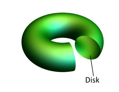
Now  are coordinates of the element of the group. Of course we would like to know how they relate to coordinates that we have introduced in the group SU(1,1). For instance in Right circular orbits in SU(1,1) we were representing SU(1,1) as a torus. How our new parameters relate to the parameters of the torus?
To answer this question we need to Cayley transform back to SU(1,1) and then express  and
and  of the torus in terms of of the NAK decomposition. I did it, using any algebraic software it is a simple task. The end result is that is the same (that is why I have chosen NAK instead of KAN, while is an algebraic function of
  . With
  we have:
(5) 
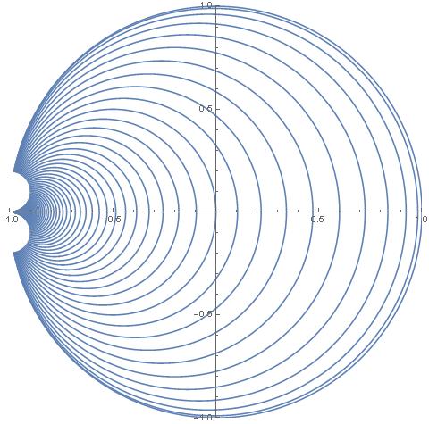
Thus after Cayley transform to SU(1,1) become coordinates on the unit disk – the cross-section of the torus. Here are their lines transformed to the disk:

 on the disk (
 fixed)
 on the disk ( fixed)
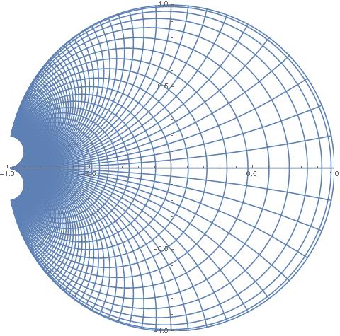 and on the disk


Thanks!