In the last note Geodesics on the upper half-plane – Part 1 Killing vectors we verified that SL(2,R) transformations are isometries of the upper half-plane endowed with the Riemannian metric defined by the line element
(1) 
The corresponding scalar product between tangent vectors being
(2) 
The idea is to use a “classical result” from differential geometry (a version of Noether’s theorem) that we have quoted from the online book by Sean Carroll:
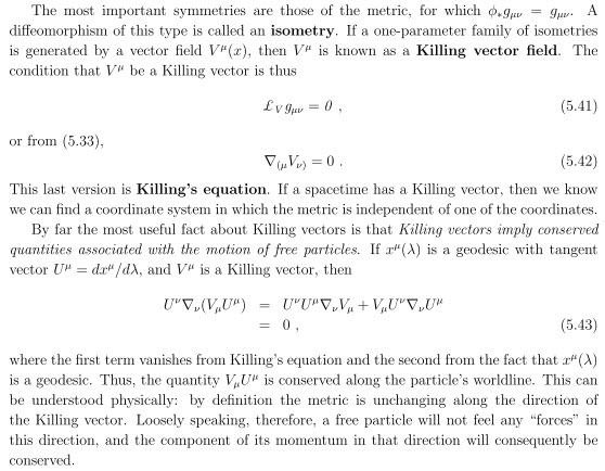
Before applying this theorem to our case let us first see how it works for the standard plane Euclidean geometry. Translations are certainly isometries there. Streamlines of the vector fields generating horizontal and vertical translations form a square grid.
That straight lines intersect these grid lines under a constant angle is evident. In fact, that could serve as an alternative definition of a straight line.
So far so good.
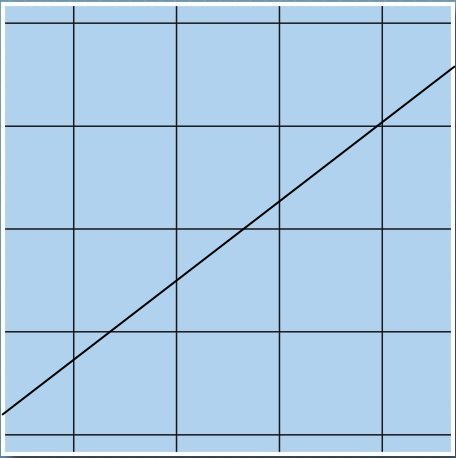
But rotations are also isometries of the Euclidean geometry.

Looking at the image that shows the intersections of a straight lines with streamlines of the vector field generating rotation – nothing is evident. The angle of intersection is certainly not constant. We have to look at the theorem more closely.
The theorem states that the scalar product between Killing vector field (generating isometry) and the tangent vector to the geodesic is constant.
A general straight line  on the plane has equation:
(3) 
The tangent vector  has components
Rotation is defined by
(4) 
The corresponding vector field  is obtained by taking derivatives with respect to
  at
at 
(5) 
It is streamlines of this vector field that we have drawn in the figure above.
Let us now calculate the scalar product of  and the vector tangent to our straight line at a point
  on our line:
(6) 
Somewhat miraculously the non-constant ( -dependent) terms have cancelled out, and the scalar product is indeed constant. Not so evident, but nevertheless true. Perhaps there is some simple argument predicting this result, but I do not know it. Either use Noether’s theorem, or use direct calculation as above.
Let us now move from the Euclidean geometry of the plane to the hyperbolic geometry of upper half-plane. In SL(2,R) generators and vector fields on the half-plane we have focused our attention on two Killing vector fields (now we know that they are “Killing”), we will call them  here:
here:
(7) 
The first one corresponds to horizontal translation, the second one to uniform dilation. Their streamlines are
Suppose now is a geodesic, with tangent vector  Its scalar products with
  and
and  should be constant. But now we remember that in calculating the scalar product we must use Eq. (2), so there will be denominator:
(8) 
(9) 
Their ratio should be therefore constant:
(10) 
(11) 
This looks rather simple. In fact it should remind us about the equation of a circle. A circle with center on some point  on
on  -axis and radius
  has equation:
(12) 
Assuming  and differentiating with respect to we get
(13) 
or
(14) 
This is exactly Eq. (11)
Thus: geodesics are circles. Or better: straight lines are circles! In fact: half-circles, because their centers are on the x-axis, and our arena is only upper half-plane.
Except that we have missed some solutions. In Conformally Euclidean geometry of the upper half-plane there was the following sentence:
In the next note we will start calculating “straight lines”, or “geodesics” of our geometry. Some of them are almost evident candidates: vertical lines, perpendicular to the real line. But what about the other ones?
Well, we have these other ones, but how the vertical lines fit our reasoning above?
This is a homework. It is somewhat tricky though ….


“The theorem states that the scalar product between Killing vector field (generating isometry) and the tangent vector to the geodesic is constant.”
Scalar product depends on tangent vector length so which one of tangent vectors do we choose?
Very good and important observation. This question will be addressed at length in the following note.
Thanks for the errata.
Homework
Vertical line parametrized as:
 const,

satisfies constant scalar product.
(Is it that trick?)
Unbelievable! And I was just writing the new post being sure that the trick will not be discovered!
Anyway I am waiting for your new post.
It is not clear to me if there exists parametrization of any curve to achieve constant scalar product (or not to achieve)?
I think the story is this: if you have only one Killing field, then “yes” (at least locally). But if you have as many linearly independent Killing fields as there are dimensions of space (two in our case), then the answer is “no”. Then the curve must be geodesic. I do not have a general proof of this, but I think it should not be too difficult.