We are still traveling in the land of 4D butterflies made of remarkable circles such as those introduced in the note Meeting with remarkable circles three days ago. We did not travel too far during these three days, but we managed to familiarize ourselves with one particular family of these peculiar creatures in the last post Being a 4D butterfly – how does it feel? It was supposed to be an illustration of More than one path, which I illustrated with the wisdom of Miyamoto Musashi, expert Japanese swordsman and rōnin:

But, in fact, my many geodesics 4D butterfly picture of yesterday did not fit the Buddhist philosophy of many paths to the top of the mountain:
What we see are many paths, all of the same type, but each leading to similar, but a different mountain. It is, perhaps, a proper illustration for the saying that:
It sounds amusing, but, as you can read in Don’t think of a black cat” by Peter Wright,

Every scenario or paradigm and situation should have a goal or a collection of goals, outcomes that are worked towards. Without goals everything is a propos of nothing (as with Dirk and Deke … or maybe All I Wanna Do by Sheryl Crow).
All I Wanna DoSheryl Crow
This ain’t no country club
And it ain’t no disco
This is New York City
1, 2, 1, 2
“All I wanna do is have a little fun before I die, ”
Says the man next to me out of nowhere
It’s apropos of nothin’
He says, “His name is William”
But I’m sure he’s Bill or Billy or Mac or Buddy
And he’s plain ugly to me
And I wonder if he’s ever had a day of fun in his whole life
…
I promised to explain in detail how exactly the 4D butterfly is created. If only to have some fun. Yesterday I was not completely sure that my idea was good. Today I think it is OK, therefore worth sharing.
The key is the algorithm described in Meeting with remarkable circles. It produces a path  in the 3D sphere in 4D space, the 3-sphere of quaternions of unit length. The function is a very particular solution of the evolution equation for a free rigid body rotating in zero-gravity space about its center of mass – like in Dzhanibekov effect. It is a very special solution, with just one flip, and also with time origin
  arranged so, that it is exactly in the middle of the flip, between one story of almost uniform rotation one way in the past, and another story of almost uniform rotations, another way, in the future. For our particular path we have
(1) 
The function is a solution of the quaternion evolution equation (cf. Quaternion evolution)
(2) 
where  and
and  is a solution of Euler’s equations:
(3) 
There are two simple ways in which we get, from our particular solution  other solutions. The first way is to multiply by a constant unit quaternion
  If is a solution, then
  is another solution. This follows by multiplying both sides of Eq. (2) by
  form the left, and by noticing that
  being constant, enters under the symbol of differentiation
  indicated by the dot over
The second method is by shifting the origin of time. For any fixed  the function
  is also a solution of Eq. (2) if is. Formally it follows from the rule of differentiation of a composite function (the Chain rule) and from the fact that
For producing the family of solutions used in the 4D butterfly image we use both methods as follows. Let
 be defined as follows:
(4) 
Then, for any fixed  the function
  is a solution of Eq. (2) with the property that
  that is all trajectories have the same origin, namely
  In verifying this last property we use the fact, that
  are unit quaternions, therefore
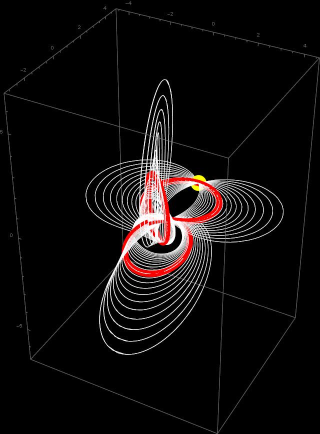
To produce the butterfly on the picture above I used from  to
to  with step
  Today I went further on, with between
  and
and  step
step  , to produce this image:

An interesting symmetry shows up when looking from far away, between circles that are “bridges”and circles that are “attractors”.
Some mystery is hidden there, waiting for being discovered in the future.
But, all of the above was in the spirit of “Happiness is a journey, not a destination” philosophy. What about many paths to the top of the mountain?
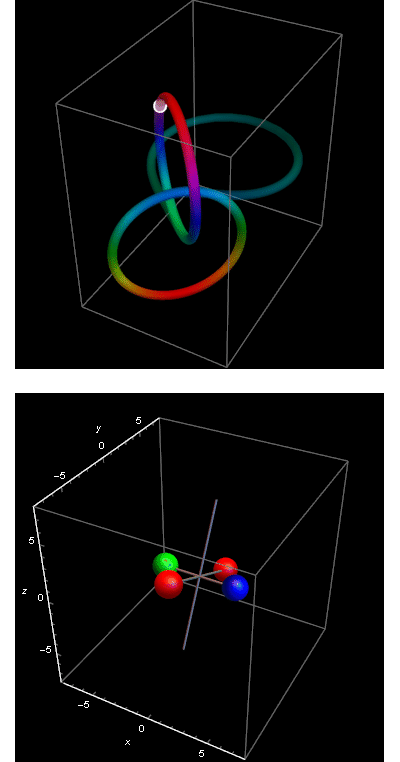
That would be keeping the attractor circles fixed (these are the two tops of mountain, one in the past, one in the future), and changing only the bridges connecting these limit circles.
This is, in fact, much easier. We just shift the time origin, and skip the part of multiplication from the left. Here are images produced this way.


The two eternal return circles are the same, only the bridges connecting them are shifting.
This last image resembles images from more realistic Dzhanibekov’s many-flips histories. It is time now to study them… if only to have some fun.
 in the quaternion group
  Consider all trajectories
  Or, better, with the property that
  Why
Why  is better? Because under stereographic projection
  is mapped into infinity, while
  We know that every trajectory is a solution of the equation


 They are special, they encode the essence of the flip in Dzhanibekov effect. In what follows, to simplify the notation I will write
  instead of


 cancels out and we get

 must be special:
 we should have

 and on the trajectory where
  the constants that enter the solution have values
 and
and 


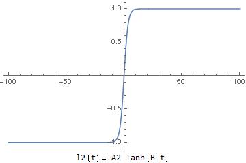
 we have
  smaller than
  and for
  smaller than
  We can consider it being zero for all practical purposes.
 it becomes practically constant and equal 1 for
  and
and  for
for 


 we have


 divided by
  We see that the “future circle” is in the plane
  while the past circle in the orthogonal plane
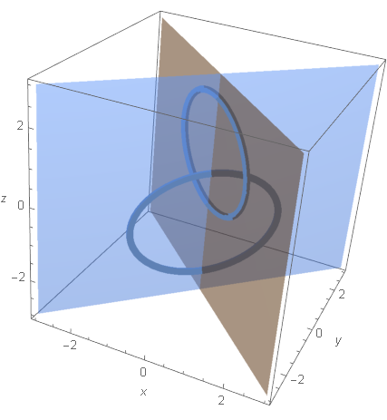
 while “the past circle” has the origin at
  Both circles have radius
 eternal return”.