The last note ended with the following problem:
Thus: geodesics are circles. Or better: straight lines are circles! In fact: half-circles, because their centers are on the x-axis, and our arena is only upper half-plane.
Except that we have missed some solutions. In Conformally Euclidean geometry of the upper half-plane there was a sentence:
In the next note we will start calculating “straight lines”, or “geodesics” of our geometry. Some of them are almost evident candidates: vertical lines, perpendicular to the real line. But what about the other ones?
Well, we have these other ones, but how the vertical lines fit our reasoning above?
If  is a vertical line, then
  therefore
  In Geodesics on the upper half-plane – Part 2 circles we arrived at equations
(1) 
(2) 
and took the ratio of the second to the first. But for vertical lines taking the ratio is not allowed. The first equation is satisfied with the constant on the right hand side equal to zero. The second equation reduces to
(3) 
If we now recall Eq. (2) from Conformally Euclidean geometry of the upper half-plane :
(4) 
we see that  and
and  on the vertical line must be proportional:
(5) 
Whenever this last equation holds, one says that  is an “affine parameter”: it is proportional to the arc length, possibly translated. In fact that is part of the definition of the geodesic that enters the “Noether’s theorem” that we are using. Usually we choose the proportionality constant equal to one.
Of course we can use Eq. (3) in order to determine the parameter  Choosing the constant equal to 1, we have
(6) 
therefore
(7) 
To my surprise Bjab has discovered this all by himself – see the discussion under the previous post
Therefore, when discussing geodesics, we will assume that they are always parametrized by their arc length or, in other words, that the tangent vector  is of unit length. In our case that is equivalent to
(8) 
Remark: There are many important examples of pseudo-Riemannian metrics, that are not positive definite. In such a case “length square” along a geodesic line is normalized to
or
or
, so that there are three kinds of geodesics. In physics this happens for space-time metrics with Minkowski signature, and in multi-dimensional Kaluza-Klein theories. We will discuss another such case in the following posts.
We can now use these insights also in the case of circular geodesics. Before we have taken the ratio of two “conservation law” equations (1,2). Now, that we know we have a circle, we can write circle equation
(9) 
where  is some function of the arc length parameter
  , and substitute into Eqs. (1,2).
(10) 
therefore Eq. (8) reduces to
(11) 
It is now a straightforward exercise to verify that with Eqs. (9–11) equations (1,2) are satisfied automatically.
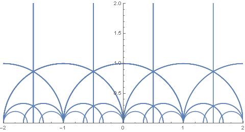
Now that we know geodesics on the upper half-plane, we can draw them for pleasure. There is a famous pattern known as Dedekind’s tesselation
I was able to reproduce a part of it, namely the part described on p. 3 in the paper on SL(2,Z) by Keith Conrad
But I would like to be able to reproduce the pretty image from website of Jerzy Kocik from Southern Illinois University

And I do not know yet how to do it.
Update: After several hours I managed to produce this:
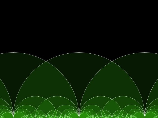


Thanks!