In the last post, Geodesics of left invariant metrics on matrix Lie groups – Part 1,we have derived Arnold’s equation – that is a half of the problem of finding geodesics on a Lie group endowed with left-invariant metric.
Suppose  is a Lie group, and
  is a scalar product (i.e. a nondegenerate bilinear form) on its Lie algebra
  . Then, using left translations
  defines a left invariant (Riemannian or pseudo-Riemannian) metric on the whole group
  If
If  is a path in
  we use left translations to define the image
  of the tangent vector
  in
in
(1) 
Usually it is written more carefully, using  instead of
  , but I am using a simplified notation, well adapted to dealing with problems for matrix groups.
If  is a geodesic for the metric , then satisfies the Arnold’s equation
(2) 
where
![\[B:Lie(G)\times Lie(G)\rightarrow Lie(G)\]](http://arkadiusz-jadczyk.eu/blog/wp-content/ql-cache/quicklatex.com-de2ba530a6f87a775ddef797d2f4145b_l3.png "Rendered by QuickLaTeX.com")
is defined as
(3) 
and  are the structure constants of , that is
(4) ![\begin{equation*}[\xi_i,\xi_j]=C_{ij}^k\, \xi_k\end{equation*}](http://arkadiusz-jadczyk.eu/blog/wp-content/ql-cache/quicklatex.com-692bc7890c932450b9207ae167292b0c_l3.png "Rendered by QuickLaTeX.com")
where  form a basis for and
(5) 
Equation (2) is a system of nonlinear ordinary differential equations with constant coefficients. In this form it can be found in Arnold’s 1966 paper “Sur la g\’eom\’etrie differentielle des groupes de Lie de dimension infinie et ses applications \`a l’hydrodynamique des fluides parfaits”, Ann. Inst.
Fourier (Grenoble) 16 (1966), 319-361.

In his blog post “The Euler-Arnold equation” Terrence Tao mentions that some people call this equation the “Euler-Arnold” equation, while some other prefer to skip Arnold’s name completely and call it “Euler-Poincare equation”. Go-figure!
Solving equations (2) is just one half of the whole problem of finding a geodesic. Once  are known, we need to solve the linear differential equation with variable coefficients that results from the definition of
  (??):
(??):
(6) 
For the case of the rotation group and free rigid body we did it in Taming the T-handle continued.
B. Kolev in his paper “Lie groups and mechanics. An introduction” shows that for the rotation group O(n) the equations of motion for the free rigid body are completely integrable. We will not need this result, but is useful to know that in general case there are always two quadratic constants of motion corresponding to “kinetic energy” and “square of the angular momentum”. We were discussing these constants of motion for the group O(3) in
“Asymmetric Spinning Top – The Hardest Concept To Grasp In Physics” – they are used in so-called Poinsot construction. We will discuss a version of it for the group O(2,1) in the future.
The first observation is that the “kinetic energy”  is, in fact, a constant, independent of
  To see that this is the case, we differentiate:
(7) 
In the previous post we wrote Eq. (2) as
(8) 
Substituting into Eq. (7) we get
(9) 
The result is zero because  is antisymmetric in
  while
while  is symmetric. That is an often used property: if
  and
and  then the contraction
  Indeed
  where in the last equality we have exchanged dummy indices names
  . If a number is equal to its negative, it must be zero.
To get the formula for the second quadratic invariant we need to return to the Ad-invariant scalar product that we have denoted  in Killing vectors, geodesics, and “Noether’s theorem”:
(10) 
The fact that is Ad-invariant implies an important relation between the matrix  and the structure constants
that we are going to use. Ad-invariance means that:
(11) 
for all  and
and 
Differentiating at  we get
(12) ![\begin{equation*}\mathring{g}([\eta,\xi_1],\xi_2)+\mathring{g}(\xi_1,[\eta,\xi_2])=0.\end{equation*}](http://arkadiusz-jadczyk.eu/blog/wp-content/ql-cache/quicklatex.com-ad385731e64a6f510be923c32b169f9f_l3.png "Rendered by QuickLaTeX.com")
Setting  we get
(13) 
Multiplying both sides by  we obtain
(14) 
We can now derive the second conservation law. The angular momentum  is defined as
(15) 
Notice that  is a covector, a one-form on , it is in the dual
  of
of  It is the metric that connects the space to its dual. While vectors in play an active role, they generate transformations, elements in the dual, one-forms from , are “passive”, they evaluate vectors to numbers. It is the metric that is the third element here, that allows the active principle to connect to the passive principle. The metric depends on the mass distribution. In application to rigid bodies the inertia tensor is encoded in the metric on the rotation group.
The second conservation law states that the square of the angular momentum evaluated with the Ad-invariant metric is constant:
(16) 
To verify we differentiate and use Eq. (8) rewritten as
(17) 
(18) 
Now, according to Eq. (14)  is antisymmetric in
  , while the product
  is symmetric, therefore we get zero:
(19) 
In the following posts we will first return to the case of the rotation group in three dimensions and the rigid body, and then try to apply a similar reasoning to the case of the Lorentz group O(2,1) in 2+1 dimensions.


 in the 3D sphere in 4D space, the 3-sphere of quaternions of unit length. The function

 and
and  is a solution of Euler’s equations:
 other solutions. The first way is to multiply
  If
If  is another solution. This follows by multiplying both sides of Eq. (
 form the left, and by noticing that
  being constant, enters under the symbol of differentiation
  indicated by the dot over
 the function
  is also a solution of Eq. (
 be defined as follows:
 the function
  is a solution of Eq. (
 that is all trajectories have the same origin, namely
  In verifying this last property we use the fact, that
  are unit quaternions, therefore
 to
to  with step
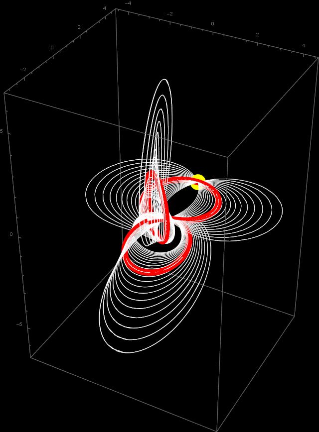
  Today I went further on, with
  and
and  step
step  , to produce this image:


 and on the trajectory where
  the constants that enter the solution have values
 and
and 


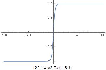
 we have
  smaller than
  and for
  smaller than
  We can consider it being zero for all practical purposes.
 it becomes practically constant and equal 1 for
  and
and  for
for 


 we have


 divided by
  We see that the “future circle” is in the plane
  while the past circle in the orthogonal plane
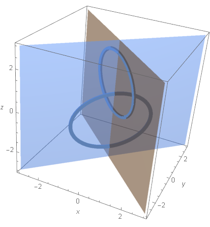
 while “the past circle” has the origin at
  Both circles have radius
 eternal return”.