I noticed that somehow I did not finish with the case So today, without further ado, I am posting the algorithm.
We have the body with and we are considering the case with , where is, as always, the ratio of the doubled kinetic energy to angular momentum squared.
Then we define
(1)
(2)
(3)
(4)
(5)
(6)
(7)
(8)
(9)
I use the above formulas to draw a stereographic projection of one particular path. So, I take , and do the parametric plot of the curve in
with
I show below two plots. One with and one with For this selected value of the time between consecutive flips, given by the formula
(10)
So, for we have somewhat less than 200 flips, and the lines are getting rather densely packed in certain regions.
Notice that is just one geodesic line, geometrically speaking the straightest possible line in the geometry determined by the inertial properties of the body.
It is this “geometry”that will become the main subject of the future notes. Geodesic line for t between -1000 and 1000 Geodesic line for t between -10000 and 10000
The last post was about The final answer for the Universe in which m>1. Yet, as I see it today, it was neither complete nor final. It was a very bad approximation. It may be also that our universe is also a very bad approximation to the one that has been intended. But that is another story. I think I will return to this problem in my blogging, but now I will concentrate on the algorithm for the rotation matrix. At the same time I will make a comment how the algorithm from the last post, for the quaternions, should be improved. The fact is that I was making wrong assumptions in my mind. Making wrong assumptions, without being conscious of the fact that one is making such assumptions, that is very dangerous. Lot of bad things happens around us for this reason…. The result of wrong assumptions
So, here is the code:
The case
The solution of the Euler’s equations has two trajectories. For one with we take
(1)
while for the other one, with we take
(2)
Let
(3)
The solution of the Euler’s equations is given by
(4)
With constants and defined as
(5)
(6)
we set the phase variable as
(7)
where the Jacobi function is defined as
Let
(8)
(9)
Then the attitude matrix is given by
(10)
If you compare this with the formulas I gave yesterday, you will find the following important difference: now I am playing with signs in the constants rather than with the signs in formulas for It took me whole day to realize that this way is a better way. I was not realizing before that there is one sign in the formula for that depends on the trajectory we are taking. The constant does this job now.
In a couple of days I will also change the formulas in the quaternionic algorithm to make them universal as well.
Now, I check the modified example3. The modified initial data in init_example3.dat file are as follows:
1.0000000000D0
10.0000000000D0
-0.544332842491675D0
0.729131780907662D0
-0.414811526666455D0
1.000000000000000D0
0.000000000000000D0
0.000000000000000D0
0.000000000000000D0
1.000000000000000D0
0.000000000000000D0
0.000000000000000D0
0.000000000000000D0
1.000000000000000D0
1.000000000000000D0
1.012686988782515D0
3.306237422473038D0
5
They are the same as in the quaternionic case discussed yesterday. The initial attitude matrix is the identity matrix. We get the same I use Mathematica to calculate the transposed final
And it seems that our code is doing the same job as the Fortran code from the giants!
Yet, as I said at the beginning, it took me the whole days to figure it out why for some initial data I was in agreement, but for another initial data there was a disagreement.
There is one little plus of the code above. The coefficient in front of is fixed, and equal ! Zanna and Celledoni in their paper and in their code have complicated formulas for this coefficient. It would take some work to verify that their complicated formula simplifies to I hope I am right here….
This is not an independent post or note or whatever. It is a continuation. In fact it is the continuation of Approaching the ultimate answer for m<1. We have approached enough. We are ready.
There was a moment’s expectant pause while panels slowly came to life on the front of the console. Lights flashed on and off experimentally and settled down into a businesslike pattern. A soft low hum came from the communication channel.
“Good morning,” said Deep Thought at last.
“Er … good morning, O Deep Thought,” said Loonquawl nervously, “do you have … er, that is …”
“An answer for you?” interrupted Deep Thought majestically. “Yes. I have.”
The two men shivered with expectancy. Their waiting had not been in vain.
“There really is one?” breathed Phouchg.
“There really is one,” confirmed Deep Thought.
Douglas Adams, The Hitchhiker’s Guide to the Galaxy
We did not get to the answer yesterday, but today is the day. We will be using the formulas from the last post. Here they are again, repeated for your convenience:
The case
(1)
The solution of the Euler’s equations has two trajectories: one with is given by
(2)
while the other one, with is given by
(3)
With constants and defined as
(4)
(5)
we set the phase variable as
(6)
where the Jacobi function is defined as
Then the quaternionic attitude solution is given by with
(7)
We consider Example Four with
(8)
(9)
is negative, the therefore we take option as in Eq. 3). We calculate that reproduces the initial angular momenta. The method is known from the previous posts:
(10)
(11)
So we have At our angular momentum is the same as angular momentum in example 4 at We calculate from Eq'(7)
(12)
thus
(13)
We verify that we have indeed a unit quaternion:
Thus the inverse quaternion is the same as conjugated one:
In the Example 4 the initial quaternion, at is . Therefore in order for our solution to reproduce the initial data of the example we set
(14)
The final time in Example 4 is Therefore we calculate
(15)
where the multiplication is the quaternion multiplication.
Calculated with Mathematica the answer is
(16)
The result from the Fortran code in the file out_example4.dat is
It seems that therefore that we have obtained the ultimate answer. At least for quaternions. We need to get it also for rotation matrices. So the saga will continue.
 So today, without further ado, I am posting the algorithm.
 and we are considering the case with
  , where
  is, as always, the ratio of the doubled kinetic energy to angular momentum squared.


 , and do the parametric plot of the curve
  in
in 
![\[\mathbf{r}(t)=\left(\frac{q_1(t)}{1-q_0(t)},\frac{q_2(t)}{1-q_0(t)},\frac{q_3(t)}{1-q_0(t)}\right).\]](http://arkadiusz-jadczyk.eu/blog/wp-content/ql-cache/quicklatex.com-9e9586446344017cc3859d919f8f5e33_l3.png "Rendered by QuickLaTeX.com")
 and one with
  For this selected value of
  the time between consecutive flips, given by the formula
 we have somewhat less than 200 flips, and the lines are getting rather densely packed in certain regions.
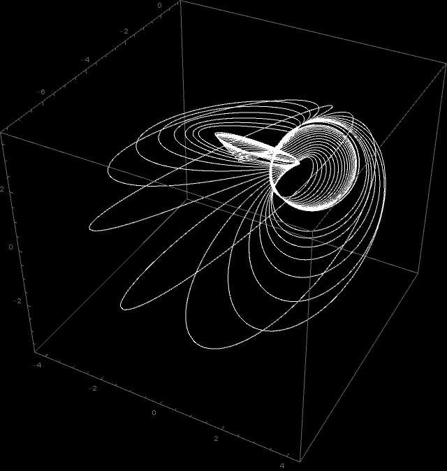


 of the Euler’s equations has two trajectories. For one with
  we take

 we take


 and
and  defined as

 as
as
 is defined as


 is given by
 rather than with the signs in formulas for
  It took me whole day to realize that this way is a better way. I was not realizing before that there is one sign in the formula for
  does this job now.
  I use Mathematica to calculate the transposed final
 is fixed, and equal
  ! Zanna and Celledoni in their paper and in their code have complicated formulas for this coefficient. It would take some work to verify that their complicated formula simplifies to


 with
with


 is negative, the therefore we take option as in Eq.
  that reproduces the initial angular momenta. The method is known from the previous posts:

 our angular momentum is the same as angular momentum in example 4 at
  We calculate
  from Eq'(
![\[q_0=W(t_0)+X(t_0)\,\mathbf{i}+Y(t_0)\,\mathbf{j}+Z(t_0)\,\mathbf{k},\]](http://arkadiusz-jadczyk.eu/blog/wp-content/ql-cache/quicklatex.com-be09436de9756e12c9ec74685b2fe1df_l3.png "Rendered by QuickLaTeX.com")


![\[||q_0||^2=W(t_0)^2+X(t_0)^2+Y(t_0)^2+Z(t_0)^2=1.0.\]](http://arkadiusz-jadczyk.eu/blog/wp-content/ql-cache/quicklatex.com-2bfa3da635c767bf601a122009646f61_l3.png "Rendered by QuickLaTeX.com")
![\[q_0^{-1}=0.435964-0.194343\,\mathbf{i}+0.0858987\,\mathbf{j}+0.874521\,\mathbf{k}.\]](http://arkadiusz-jadczyk.eu/blog/wp-content/ql-cache/quicklatex.com-e5944a30c81baa7160eec07e09534107_l3.png "Rendered by QuickLaTeX.com")
 is
is  . Therefore in order for our solution to reproduce the initial data of the example we set
 Therefore we calculate


