In Deriving invariant hyperbolic Riemannian metric on the half-plane we have calculated the line element for the SL(2,R) invariant hyperbolic geometry on the upper half-plane:
(1) 
Using this formula we can easily calculate the length of any segment of any curve. If  is a parametric equation of the curve, then
  and so
(2) 
(3) 
In this last formula we have used the fact that in the upper half-plane we have 
From the studies of geometry of surfaces and its generalization developed mainly by Riemann we know that the formula for the line element allows us not only to find the length, but also the angles.
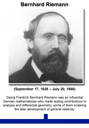
Riemannian geometry originated with the vision of Bernhard Riemann expressed in his inaugural lecture “Ueber die Hypothesen, welche der Geometrie zu Grunde liegen” (“On the Hypotheses on which Geometry is Based”). It is a very broad and abstract generalization of the differential geometry of surfaces in
 . Development of Riemannian geometry resulted in synthesis of diverse results concerning the geometry of surfaces and the behavior of geodesics on them, with techniques that can be applied to the study of differentiable manifolds of higher dimensions.
It allows us to calculate scalar products of tangent vectors. Let us rewrite Eq. (1) in the form:
![\[ds^2=\begin{bmatrix}dx&dy\end{bmatrix}\begin{bmatrix}g_{xx}&g_{xy}\\g_{yx}&g_{yy}\end{bmatrix}\begin{bmatrix}dx\\dy\end{bmatrix}= g_{xx}dx^2+2g_{xy}dx\,dy+g_{yy}dy^2,\]](http://arkadiusz-jadczyk.eu/blog/wp-content/ql-cache/quicklatex.com-942c3a90f1220596b77d711e33ad5d35_l3.png "Rendered by QuickLaTeX.com")
using the symmetric (i.e.  ) “Riemannian metric” matrix
![\[g=\begin{bmatrix}g_{xx}&g_{xy}\\g_{yx}&g_{yy}\end{bmatrix}.\]](http://arkadiusz-jadczyk.eu/blog/wp-content/ql-cache/quicklatex.com-aed021f610b4c8dc841e7b55ad71977a_l3.png "Rendered by QuickLaTeX.com")
Thus, from Eq. (1), we have 
 and
and  . Or
. Or
(4) 
In general, if  and
and  are two tangent vectors at
  then their scalar product is given by a general formula
(5) 
which in our case specializes to
(6) 
The numerator is exactly the same as for the Euclidean scalar product. It has the consequence that the angles in the hyperbolic upper half-plane geometry are the same as in the Euclidean geometry. That it is so follow from the definitions. Angles in any Riemannian geometry are defined the same way as in the Euclidean geometry. If  are two tangent vectors at
  then the angle
  between them is defined through the formula:
(7) 
where  and
and  are their norms. If we use the scalar product given by Eq. (6), then the denominator
  in
in  cancels out with the product of denominators is the norms. The end result is
(8) 
.
Therefore, when we look at the picture like the one obtained in the last post:

all hyperbolic geometry angles between various lines at any particular joining point are the same as the perceived ones by our eyes ones – contrary to the sizes, where SL(2,R) invariant geometry and Euclidean geometry we are used to are different.
Whenever we have two metrics, and  that differ a scalar factor
  we say that they are conformally related, or conformal to each other. In our case the metric in Eq. (4) is proportional to the identity matrix, our geometry is conformally Euclidean.
In the next note we will start calculating “straight lines”, or “geodesics” of our geometry. Some of them are almost evident candidates: vertical lines, perpendicular to the real line. But what about the other ones?
Our geometry is a toy geometry, as simple as possible. The group S(1,1) (or SL(2,R) ) is too simple. But one step further there is SU(2,2) – which became the basis for the “chronometric cosmology” developed by the late mathematician Irving Ezra Segal.
From American Astronomical Society, Irving Ezra Segal (1918 – 1998)
… The number of astronomers convinced was small, with experimentalists providing a slightly more favorable reception than theoreticians. Occasionally, the controversy was quite theatrical. A younger colleague of Segal was assaulted on Massachusetts Avenue by an astrophysicist still fuming from a Segalian conversation, and the publication of all the correspondence to and from Cambridge would be delightful. Particularly vituperative referee reports were always posted on his office door, some years overflowing onto the walls. Tee-shirts emblazoned with “Save Energy—Stop the Expansion of the Universe” can still be seen in Harvard Square. Whatever the final judgment is on the chronometric theory, Segal’s contributions to mathematics and mathematical physics have already had profound influence. Segal will be remembered for his conviction that the proper role of mathematics is to illuminate physics and his constant, irascible charm. We will also remember the perfect host, pouring wine for many a dinner, discussing physics, mathematics, philosophy, the proper preparation of coffee, and life.


by the late mathematician ->
?
Some mathematicians are late mathematicians:
John Nash: Why the late mathematician had such A Beautiful Mind
…
Nash died on May 23 (2015) after a car accident on the New Jersey Turnpike. His wife Alicia Nash, who cared for him, also passed away in the collision. It is believed that the couple had not worn their seatbelts.
Or, in New Foundations for Classical Mechanics by David Hestenes:
“The prevailing attitude toward quaternions is exhibited in a biographical sketch of Hamilton by the late mathematician E. T. Bell.”
The obituaries for Segal were interesting,
http://www.tony5m17h.net/SegalConf3.html#Segalobits
Bertram Kostant said, in his Segal obituary article:
“… I have it from a highly reliable but unnamed source that there is a growing group of cosmologists who have come to believe that the correct understanding of the redshift is some sort of fusion of the Doppler effect and Irving’s theory. So it is not impossible that Irving could turn out to be correct after all. …”.
I asked Bertram Kostant about that quote, and he said that he did not name the source because the source requested anonymity because he (the source) wanted to avoid entanglement in the heated controversy that surrounds Segal’s redshift ideas. I think that it is regrettable that interesting scientific ideas become so involved in unpleasant controversy that competent people become intimidated from discussing such ideas. As to how and why Segal’s ideas became controversial, Edward Nelson, in his Segal obituary article, said:
“… Part of the reason lies in Segal’s style of scientific exchange – at times it resembles that of Giordano Bruno (later burned at the stake), who very shortly after his arrival in Geneva issued a pamphlet on Twenty Errors Committed by Professor De la Faye in a Single Lesson. But part of the fault lies with cosmologists and particle physicists intent on defending turf. …”.
Thanks for these insights.
Fixed. Thanks.
Ponieważ w dalszym ciągu nie wiem co jest desygnatem Twojego “late mathematician” zapytam w natywnym języku:
Czy “late mathematician” to
1. spóźniony matematyk,
2. opóźniony w rozwoju matematyk,
3. lekki matematyk,
4. leciwy matematyk,
5. niedoszły matematyk,
6. niespełniony matematyk,
7. słaby matematyk,
8. nieżyjący matematyk,
9. świętej pamięci matematyk
10. …….. ?
Mój słownik polsko angielski pod hasłem “zmarły” ma taki przykład “mój zmarły mąż” – “my late husband”. Więc i do matematyka to się raczej też może odnosić. Dziwny jest ten angielski. Bo o spóźnionych matematykach też by można: http://unclejokes.com/jokes/recentjokes/7124/late-mathematician
Late Mathematician
A mathematician wandered home at 3 AM. His wife became very upset, telling him, “You’re late! You said you’d be home by 11:45!” The mathematician replied, “I’m right on time. I said I’d be home by a quarter of twelve.”
Było źle podpięte (jest do Bjaba).
Delete nie działa (-1).
10. Doświadczony (itp.)?
Said the straight man to the late man
“Where have you been?”
I’ve been here and I’ve been there
And I’ve been in between
https://www.youtube.com/watch?v=s82yWPjzYCA
Thanks.