Circles of eternal return

Let me recall the particular trajectory that we are discussing. In fact the particular part of this particular trajectory where the flip occurs.


Click on the image to open gif animation. It will take time to load as it is 2.5 MB.

The flip is much like one of these flips that Russian cosmonaut Dzhanibekov observed in zero gravity, and was very much perplexed by the phenomenon.

We are investigating the jungle of math that we have to apply in order to simulate such a behavior of an ideal Platonic rigid body. At present we are analyzing the special conditions when only one flip happens. Apart of a rather short (as compared to eternity) period of time when the flip occurs, the body rotates uniformly about its middle axis. Its trajectory in the rotation group, represented by quaternions of unit norm, follows a circle. One circle before flip, another circle after the flip.

In this note I am taking a close look at these two circles. Can we find their exact coordinate representation in 3D after stereographic projection?
Yes, we can, and we will do it now.
We use the formulas from Meeting with remarkable circles.
For the body of our choice, with moments of inertia I_1=1, I_2=2,I_3=3, and on the trajectory where d=1/I_2, the constants that enter the solution have values

(1)   \begin{eqnarray*} A_1&=&\sqrt{\frac{I_1(I_3-I_2)}{I_2(I_3-I_1)}}=1/2,\\ A_2&=&1,\\ A_3&=&\sqrt{\frac{I_3(I_2-I_1)}{I_2(I_3-I_1)}}=\frac{\sqrt{3}}{2},\\ B&=&\frac{1}{I_2}\,\sqrt{\frac{(I_2-I_1)(I_3-I_2)}{I_1I_3}}=\frac{1}{2\sqrt{3}},\\ \delta&=&\frac{\sqrt{I_2(I_3-I_1)}-\sqrt{I_1(I_3-I_2)}}{\sqrt{I_3(I_2-I_1)}}=\frac{1}{\sqrt{3}}. \end{eqnarray*}

In the solution of the Euler’s equations we have functions \tanh (Bt) and \mathrm{sech} (Bt)

(2)   \begin{eqnarray*} l_1(t)&=& A_1\,\mathrm{sech }(B t),\\ l_2(t)&=&A_2\,\tanh( B t),\\ l_3(t)&=&A_3\,\mathrm{sech }(B t), \end{eqnarray*}

with \mathrm{sech }(x)=1/\cosh(x).
Here are the plots of these functions:
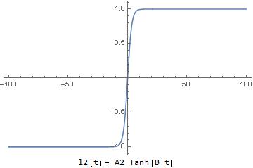

For |t|>100 we have l_1(t) smaller than 10^{-12}, and for |t|>200 smaller than 10^{-25}. We can consider it being zero for all practical purposes.
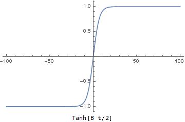
As for l_2(t), it becomes practically constant and equal 1 for t>100, and -1 for t<-100.
We then have the function \psi(t)

(3)   \begin{equation*} \psi(t)=\frac{t}{I_2}+2\arctan\left(\delta \tanh(B t/2)\right).  \end{equation*}

Again for all practical purposes for t>100 we have

(4)   \begin{equation*}\psi(t)\approx  t/2+\pi/3,\end{equation*}

and for t<-100,

(5)   \begin{equation*}\psi(t)\approx  t/2-\pi/3.\end{equation*}

Let us substitute these formulas into the solution for q(t)

(6)   \begin{eqnarray*} q_0(t)&=&\frac{\sqrt{1+l_1(t)}\cos\frac{\psi(t)}{2}}{\sqrt{2}},\\ q_1(t)&=&\frac{\sqrt{1+l_1(t)}\sin\frac{\psi(t)}{2}}{\sqrt{2}},\\ q_2(t)&=&\frac{l_3(t)\cos\frac{\psi(t)}{2}+l_2(t)\sin\frac{\psi(t)}{2}}{\sqrt{2(1+l_1(t))}},\\ q_3(t)&=&\frac{-l_2(t)\cos\frac{\psi(t)}{2}+l_3(t)\sin\frac{\psi(t)}{2}}{\sqrt{2(1+l_1(t))}}. \end{eqnarray*}

We obtain

(7)   \begin{eqnarray*} q_0(t)&=&\frac{\cos\frac{\psi(t)}{2}}{\sqrt{2}},\\ q_1(t)&=&\frac{\sin\frac{\psi(t)}{2}}{\sqrt{2}},\\ q_2(t)&=&\pm\frac{\sin\frac{\psi(t)}{2}}{\sqrt{2}},\\ q_3(t)&=&\frac{\mp\cos\frac{\psi(t)}{2}}{\sqrt{2}}. \end{eqnarray*}

The upper signs concern t>100 the lower signs concern t<-100.
In stereographic projection we are plotting (q_1,q_2,q_3) divided by 1-q_0. We see that the “future circle” is in the plane x=y, while the past circle in the orthogonal plane x=-y.

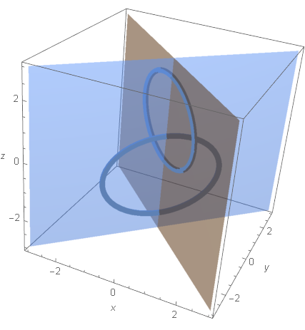
I did my geometric exercises and I have found that “the future circle” has origin at (0,0,-1), while “the past circle” has the origin at (0,0,1). Both circles have radius \sqrt{2}.

So, we have complete information about these “circles of eternal return”.
One more comment: in Another geodesic line I was showing what I thought was a subtle structure of the trajectory approaching the circle:

But now I know that it was a numerical artefact. As noticed in today’s post, for |t|>100 computer will see only one line, no fine structure. To be sure I asked my computer to take more points on the plot (100000 instead of 10000) and all the fine structure disappeared.

Meeting with remarkable circles

According to the web site “How stuff works”

Our universe is devoid of perfect circles.

Only in the abstract world of pure mathematics can we find our perfect circle — a world of points and infinitely-thin lines with no room for particle inconsistencies or spherical oblateness.

In our world there is no true beauty, but we have an innate understanding and longing for the true form of beauty as it exists beyond the limits of our reality. There’s no true justice here, but we have a sense of it because the unreachable ideal exists in the realm of forms.

And this is what we are after: the true beauty. And nothing is going to stop us. Here it is. We stumbled upon it in our analysis of the internal mathematical structure of the Dzhanibekov effect. It is one of the simplest and at the same time one of the most amazing effects hidden in the laws of physics that were in principle known for centuries, but there is a difference between knowing and understanding.

In “Meetings with Remarkable Men” G. I. Gurdjieff wrote:

YES, PROFESSOR, KNOWLEDGE AND UNDERSTANDING ARE QUITE DIFFERENT. Only understanding can lead to being, whereas knowledge is but a passing presence in it. New knowledge displaces the old and the result is, as it were, a pouring from the empty into the void.
One must strive to understand; this alone can lead to our Lord God.
And in order to be able to understand the phenomena of nature, according and not according to law, proceeding around us, one must first of all consciously perceive and assimilate a mass of information concerning objective truth and the real events which took place on earth in the past; and secondly, one must bear in oneself all the results of all kinds of voluntary and involuntary experiencing.

Yes, we want to know, because knowledge protects (while ignorance endangers), but we also want to understand. For that math is needed. Here are, one more time, our remarkable circles, now rotating in front of you as in the Spring Fashion Show.

Click on image to start the rotation animation

These are the two remarkable limit circles connected by the bridge.

And how do we get these limit circles?

Simple we go to the limits.

Recall the formulas from The mysterious paths on the three-sphere. Remember, we set I_1=1,\,I_2=2,\,I_3=3.

(1)   \begin{eqnarray*} A_1&=&\sqrt{\frac{I_1(I_3-I_2)}{I_2(I_3-I_1)}}=1/2,\\ A_2&=&1,\\ A_3&=&\sqrt{\frac{I_3(I_2-I_1)}{I_2(I_3-I_1)}}=\frac{\sqrt{3}}{2},\\ B&=&\frac{1}{I_2}\,\sqrt{\frac{(I_2-I_1)(I_3-I_2)}{I_1I_3}}=\frac{1}{2\sqrt{3}},\\ \delta&=&\frac{\sqrt{I_2(I_3-I_1)}-\sqrt{I_1(I_3-I_2)}}{\sqrt{I_3(I_2-I_1)}}=\frac{1}{\sqrt{3}}. \end{eqnarray*}

Define:

(2)   \begin{eqnarray*} l_1(t)&=& A_1\,\mathrm{sech }(B t),\\ l_2(t)&=&A_2\,\tanh( B t),\\ l_3(t)&=&A_3\,\mathrm{sech }(B t), \end{eqnarray*}

where \mathrm{sech }(x)=1/\cosh(x).
Define

(3)   \begin{equation*} \psi(t)=\frac{t}{I_2}+2\arctan\left(\delta \tanh(B t/2)\right). \end{equation*}

Define:

(4)   \begin{eqnarray*} q_0(t)&=&\frac{\sqrt{1+l_1(t)}\cos\frac{\psi(t)}{2}}{\sqrt{2}},\\ q_1(t)&=&\frac{\sqrt{1+l_1(t)}\sin\frac{\psi(t)}{2}}{\sqrt{2}},\\ q_2(t)&=&\frac{l_3(t)\cos\frac{\psi(t)}{2}+l_2(t)\sin\frac{\psi(t)}{2}}{\sqrt{2(1+l_1(t))}},\\ q_3(t)&=&\frac{-l_2(t)\cos\frac{\psi(t)}{2}+l_3(t)\sin\frac{\psi(t)}{2}}{\sqrt{2(1+l_1(t))}}. \end{eqnarray*}

We want to know what happened in the distant path, and what will happen in the distant future. In other words we are interested in the asymptotic behavior at t\rightarrow +\infty and t\rightarrow -\infty.

Let us start with l_1(t).

We see that in the past and in the future l_1(t) effectively vanishes. The same for l_3(t). For l_2(t) we have:

Therefore in the past, asymptotically, \mathbf{L}=(0,-1,0), while in the future \mathbf{L}=(0,1,0).
What about \psi(t)?
Here is the plot of \tanh B t/2

And 2 \arctan \frac{1}{\sqrt{3}}=\pi/3. Therefore asymptotically, in the past,

(5)   \begin{equation*}\psi(t)=\frac{t}{2}-1.0472,\end{equation*}

and in the future

(6)   \begin{equation*}\psi(t)=\frac{t}{2}+1.0472.\end{equation*}

Therefore asymptotically at t\rightarrow -\infty

(7)   \begin{equation*}q(t)=\frac{1}{\sqrt{2}}(\cos \psi/2,\sin \psi/2,-\sin \psi/2,\cos \psi/2),\end{equation*}

while for t\rightarrow +\infty

(8)   \begin{equation*}q(t)=\frac{1}{\sqrt{2}}(\cos \psi/2,\sin \psi/2,\sin \psi/2,-\cos \psi/2),\end{equation*}

where \psi is given either by (5) or (6).
This will give us the two remarkable circles … In the next post. For now these circles should do:

Leshan Giant Buddha bridge Photography by Edy Petrova

Metamorphosis in action

Here is the deal:
There are two interlinked circles, like in a chain. You move around one of the circles for half of eternity almost without any change. Almost. Because one day you reach a threshold, there is an action potential, a quantum jump. And you move to the second circle, where you will continue for the second half of eternity.

This is the archetype, the essence, the kernel, of the Dzhanibekov effect that my series of posts is about.

The essential math is summarized in my previous post. Here comes the animation.

Click on the image to open gif animation. It will take time to load as it is 2.5 MB.

The upper image shows the unit quaternion representing the rigid body rotation. It moves first on one circle, then makes the jump to the second circle.
The lower image shows the rotating rigid body. Time on both images is synchronized. The quantum jump is the flip of the rotating rigid body.

Update: My Mathematica animation (almost the same as above) code that can be analyzed and should run with free Mathematica CDF Player (probably needs a recent one) is here.