In Texas kids learn about the number “pi” in 6th grade. I do not know how it is in Kansas. But we are not in Kansas anyway, so we can learn it now.
We are not in Texas, and we are not in Kansas. We are on the unit disk with hyperbolic geometry defined by the transitive action of SU(1,1) – as it was discussed in the recent series of posts. We know the line element:
(1)
We can now ask this pressing question: what is the ratio of the circumference of a circle to its radius?
Any point of the disk is as good as any other, but in the standard coordinates that we are using the origin of the disk is most convenient. Let us introduce polar coordinates
(2)
We need to express our line element in terms of We calculate
Consider now a circle with and running from to What is the length of its circumference? We have to integrate Going around circumference is constant, so Therefore
What is the length of its radius? Along the radius is constant, so , so
Looking at the graph of the function
we see that the ratio circumference to radius on the disk is always greater than In fact the ratio is growing faster and faster with increasing .
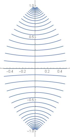
These are straight lines on the disk obtained from the interval on the real axis by the action of a one-parameter family of left shifts from SU(1,1). Since our geometry is, by definition, invariant under such transformations, all these lines are of equal length.
I thought it would be interesting to overlay these lines, obtained numerically, with Escher’s Angels and Demons picture to see how well Escher’s drawing corresponds to calculations. Here is the result:
Escher’s Angels and Demons and hyperbolic geometry
As far as I can see angels and demons do not know how to use computers. They work using intuition and aesthetic feelings. And yet Escher’s drawing corresponds to calculations almost perfectly.
We can use it to find, say, the distance of a point on the vertical axis from the origin. Tha path is paramatrized by where varies from to Therefore the length of the path
is
So, we have
(2)
For producing Fig. 1 we used the family of SU(1,1) matrices;
implements fractional linear transformation
Thus
(3)
The distance from the origin to along the vertical axis, is therefore
It follows that the parallel lines in Fig. 1 are all equidistant, if the distance between them is measured along the vertical axis.
That was our first use of the formula for the line element of the non-Euclidean hyperbolic geometry of the Poincaré disk. We will have to play with it a little bit more, so that we will not be afraid that it will bite us.
There is no geometry without metry. That is, without metric. It was Bernhard Riemann who gave the foundations to what we call today “Riemannian geometry”. When Einstein learned Rimennian geometry, he was able to compete with smart mathematicians and lay the foundations of the theory of gravitation – the General Relativity Theory.
“[In 1912] I suddenly realized that Gauss’s theory of surfaces holds the key for unlocking this mystery. I realized that Gauss’s surface coordinates had a profound significance. However, I did not know at that time that Riemann had studied the foundations of geometry in an even more profound way. I suddenly remembered that Gauss’s theory was contained in the geometry course given by Geiser when I was a student… I realized that the foundations of geometry have physical significance. My dear friend the mathematician Grossmann was there when I returned from Prague to Zürich. From him I learned for the first time about Ricci and later about Riemann. So I asked my friend whether my problem could be solved by Riemann’s theory [Pais’s italics], namely, whether the invariants of the line element could completely determine the quantities I had been looking for.”
Albert Einstein, as quoted by Abraham Pais in Subtle is the Lord, Pais’s scientific biography of Einstein.
So, it is time for us to get familiar with this “line element“. Here it is, written with the hand of Albert Einstein himself, probably in 1913, in his Zurich notebook:
We want to find our “line element” on the disk. Equivalently: we want to find the metric tensor
That is, when from a point with disk coordinates we make a small step, and arrive at the point with coordinates what will be the length of this step? If the geometry were Euclidean, and our coordinates were Cartesian, rectangular, the answer would be simple: from the Pythagoras formula. But our geometry is non-Euclidean. And we want our step length to be invariant under SU(1,1) transformations, which are non-linear on the disk. What to do?
Two fundamental errors led Einstein to reject generally covariant gravitational field equations for over two years as he was developing his general theory of relativity. The first is now well known. It was the presumption that weak, static gravitational fields must be spatially flat and a corresponding assumption about his weak field equations. I conjecture that a second hitherto unrecognized error also defeated Einstein’s efforts: he unwittingly reified his spacetime coordinate systems. The same error, months later, allowed the hole argument to convince Einstein that all generally covariant gravitational field equations would be physically uninteresting.
While doing our calculations we will try to avoid errors, at least those computational. We will listen to Gottfried Leibniz who, as mentioned in the last note, has made this advice:
“It is unworthy of excellent men to lose hours like slaves in the labor of calculation which could be relegated to anyone else if machines were used.”
As we have learned in From SU(1,1) to the Lorentz group, a point on the disk determines a point on the hyperboloid in three-dimensional space-time
Space-time hyperboloid and the Poincare disk models
When we are making a small step on the disk, we are making also a small step on the hyperboloid. Well, I am joking. When our step on the disk is very close to the boundary, the corresponding step on the hyperboloid can be “huge”. What I really mean is: when we make an infinitesimally small step …. The concept of an infinitesimally small step belongs to the calculus, and I will assume that we know how to use the elementary calculus concepts.
In the the previous post we used the formulas expressing as functions of :
(1)
From these formulas we can calculate in terms of according to the following general prescription
(2)
We can do these calculations by hand, but that would be unworthy of excellent men. Machine will do it for us. Once we know we can calculate the corresponding line element using the formula of special relativity, a generalization of the Pythagoras law from space to space-time. I our case it is now convenient to chose the signature then
(3)
I let Maxima to do the calculations using this code:
If you want, save this code as a file, say, “ds2.mac”. Install and run wxMaxima, use File/Batch File … to load the code. The answer is produced immediately:
We will yet have to find out what can we do with it? Lot of things. We can find geodesics (we have already guessed what they are), curvature …. Yes, our disk is curved even if it does not look so.

 that we are using the origin of the disk is most convenient. Let us introduce polar coordinates
 We calculate
![\[ dx =d\rho\cos \phi-\rho\sin\phi d\phi,\]](http://arkadiusz-jadczyk.eu/blog/wp-content/ql-cache/quicklatex.com-62a6097512d9d1ed135cbb9ee24ba2e5_l3.png "Rendered by QuickLaTeX.com")
![\[ dy =d\rho \sin\phi+\rho\cos\phi d\phi,\]](http://arkadiusz-jadczyk.eu/blog/wp-content/ql-cache/quicklatex.com-c5dd55b15056ea4874e8fcc576aacddc_l3.png "Rendered by QuickLaTeX.com")
![\[dx^2= d\rho^2\cos^2\phi-2\rho\sin\phi\cos\phi d\rho d\phi+\rho^2\sin^2\phi d\phi^2,\]](http://arkadiusz-jadczyk.eu/blog/wp-content/ql-cache/quicklatex.com-00ecdf09857cc43e756438ca297ab703_l3.png "Rendered by QuickLaTeX.com")
![\[dy^2= d\rho^2\sin^2\phi+2\rho\sin\phi\cos\phi d\rho d\phi+\rho^2\cos^2\phi d\phi^2,\]](http://arkadiusz-jadczyk.eu/blog/wp-content/ql-cache/quicklatex.com-28e17b7c699c5d125fee560d1b73c897_l3.png "Rendered by QuickLaTeX.com")
![\[dx^2+dy^2=d\rho^2+\rho^2 d\phi^2,\]](http://arkadiusz-jadczyk.eu/blog/wp-content/ql-cache/quicklatex.com-3429ab361a5932d733a93ae16e376cb5_l3.png "Rendered by QuickLaTeX.com")
![\[ds^2=4\frac{d\rho^2+\rho^2d\phi^2}{(1-\rho^2)^2}.\]](http://arkadiusz-jadczyk.eu/blog/wp-content/ql-cache/quicklatex.com-de0e86a0c67fd372112804208b670657_l3.png "Rendered by QuickLaTeX.com")
 and
and  running from
  to
to  What is the length
  of its circumference? We have to integrate
  Going around circumference
  is constant, so
  Therefore
![\[C=\int_0^{2\pi}ds=\int_0^{2\pi}\frac{2\rho_0 d\phi}{1-\rho_0^2}=\frac{4\pi \rho_0}{1-\rho_0^2}.\]](http://arkadiusz-jadczyk.eu/blog/wp-content/ql-cache/quicklatex.com-a141c40deee3ce2a3e732ca68ef24911_l3.png "Rendered by QuickLaTeX.com")
 of its radius? Along the radius
  , so
, so![\[r=\int_0^{\rho_0} ds=\int_0^{\rho_0}\frac{2d\rho}{1-\rho^2}=2\mathrm{arctanh}\rho_0.\]](http://arkadiusz-jadczyk.eu/blog/wp-content/ql-cache/quicklatex.com-f75be9a1c86f5baa10bb036ab268c9c5_l3.png "Rendered by QuickLaTeX.com")
![\[\rho_0=\tanh\frac{r}{2}.\]](http://arkadiusz-jadczyk.eu/blog/wp-content/ql-cache/quicklatex.com-5bd899c0ad119fa37dcf564eee83eea8_l3.png "Rendered by QuickLaTeX.com")
![\[C=4\pi\frac{\sinh(r/2)/\cosh(r/2)}{1-\sinh^2(r/2)/\cosh^2(r/2)}=2\pi\frac{2\sinh(r/2)\cosh(r/2)}{\cosh^2(r/2)-\sinh^2(r/2)}.\]](http://arkadiusz-jadczyk.eu/blog/wp-content/ql-cache/quicklatex.com-05b53a2fcb9caea7c144cfb7c8fe5641_l3.png "Rendered by QuickLaTeX.com")


 ).
).

![[-0.5,0.5]](http://arkadiusz-jadczyk.eu/blog/wp-content/ql-cache/quicklatex.com-eee378511d1ac25fd994178aa1c7c64f_l3.png "Rendered by QuickLaTeX.com") on the real axis by the action of a one-parameter family
on the real axis by the action of a one-parameter family  of left shifts from SU(1,1). Since our geometry is, by definition, invariant under such transformations, all these lines are of equal length.
 on the vertical axis from the origin. Tha path is paramatrized by
  where
where  varies from
  Therefore the length of the path
![\[ s=\int_0^{y_0} ds= \int_0^{y_0} \frac{2 dy}{1-y^2}=2|\mathrm{arctanh} (y_0)|.\]](http://arkadiusz-jadczyk.eu/blog/wp-content/ql-cache/quicklatex.com-4e37cc87675f4eb19ee1c4df3e61f761_l3.png "Rendered by QuickLaTeX.com")

![\[A_1(t)=\begin{bmatrix}\cosh(t)&i\sinh(t)\\-i\sinh(t)&\cosh(t).\end{bmatrix}\]](http://arkadiusz-jadczyk.eu/blog/wp-content/ql-cache/quicklatex.com-b58afd109b8b0bee30bdf68d18450093_l3.png "Rendered by QuickLaTeX.com")
![\[A_1(t):z\mapsto \frac{\cosh(t)z-i\sinh(t)}{i\sinh(t)z +\cosh(t)}.\]](http://arkadiusz-jadczyk.eu/blog/wp-content/ql-cache/quicklatex.com-3173c4d73a9d4b39793bc18be1b3215c_l3.png "Rendered by QuickLaTeX.com")

 along the vertical axis, is therefore
![\[s(t)=2|\mathrm{arctanh}(-\tanh(t))|=2|t|.\]](http://arkadiusz-jadczyk.eu/blog/wp-content/ql-cache/quicklatex.com-d16add9b46b1b2f16d64faac500418d9_l3.png "Rendered by QuickLaTeX.com")


 what will be the length
  of this step? If the geometry were Euclidean, and our coordinates were Cartesian, rectangular, the answer would be simple:
  from the Pythagoras formula. But our geometry is non-Euclidean. And we want our step length to be invariant under SU(1,1) transformations, which are non-linear on the disk. What to do?
 on the hyperboloid in three-dimensional space-time
 on the disk, we are making also a small step
  on the hyperboloid. Well, I am joking. When our step on the disk is very close to the boundary, the corresponding step on the hyperboloid can be “huge”. What I really mean is: when we make an infinitesimally small step …. The concept of an infinitesimally small step belongs to the calculus, and I will assume that we know how to use the elementary calculus concepts.

 then
then


