Hyperbolic Geometry | Open System - Ark's blog

From SU(1,1) to the Lorentz group

Posted on 2017/04/112017/04/22 by arkajad

From the two-dimensional disk we are moving to three-dimensional space-time. We will meet Einstein-Poincare-Minkowski special relativity, though in a baby version, with x and y, but without z in space. It is not too bad, because the famous Lorentz transformations, with length contraction and time dilation happen already in two-dimensional space-time, with x and t alone. We will discover Lorentz transformations today. First in disguise, but then we will unmask them.

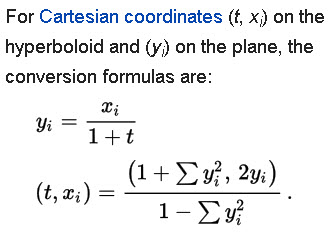
First we recall, from The disk and the hyperbolic model, the relation between the coordinates $(x,y)$ on the Poincare disk $x^2+y^2<1$ , and $(X,Y,T)$ on the unit hyperboloid $T^2-X^2-Y^2=1.$

Space-time hyperboloid and the Poincare disk models

(1) $\begin{eqnarray*} X&=&\frac{2x}{1-x^2-y^2},\\ Y&=&\frac{2y}{1-x^2-y^2},\\ T&=&\frac{1+x^2+y^2}{1-x^2-y^2}. \end{eqnarray*}$

(2) $\begin{eqnarray*} x&=&\frac{X}{1+T},\\ y&=&\frac{Y}{1+T}. \end{eqnarray*}$

We have the group SU(1,1) acting on the disk with fractional linear transformations. With $z=x+iy$ and $A$ in SU(1,1)

(3) $\begin{equation*}A=\begin{bmatrix}\lambda&\mu\\ \nu&\rho\end{bmatrix},\end{equation*}$

the fractional linear action is

(4) $\begin{equation*}A:z\mapsto z_1=\frac{\rho z+\nu}{\mu z+\lambda}.\end{equation*}$

By the way, we know from previous notes that $A$ is in SU(1,1) if and only if

(5) $\begin{equation*}\nu=\bar{\mu},\,\rho=\bar{\lambda},\quad|\lambda|^2-|\mu|^2=1.\end{equation*}$

Having the new point on the disk, with coordinates $(x_1,y_1)$ we can use Eq. (1) to calculate the new space-time point coordinates $(X_1,Y_1,T_1).$ This is what we will do now. We will see that even if $z_1$ depends on $z$ in a nonlinear way, the space-time coordinates transform linearly. We will calculate the transformation matrix $L(A),$ and express it in terms of $\lambda$ and $\mu.$ We will also check that this is a matrix in the group SO(1,2).

The program above involves algebraic calculations. Doing them by hand is not a good idea. Let me recall a quote from Gottfried Leibniz, who, according to Wikipedia

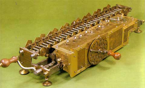
He became one of the most prolific inventors in the field of mechanical calculators. While working on adding automatic multiplication and division to Pascal’s calculator, he was the first to describe a pinwheel calculator in 1685[13] and invented the Leibniz wheel, used in the arithmometer, the first mass-produced mechanical calculator. He also refined the binary number system, which is the foundation of virtually all digital computers.

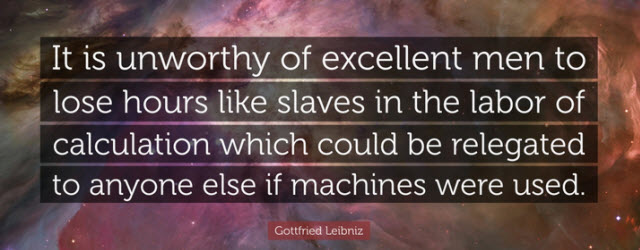
“It is unworthy of excellent men to lose hours like slaves in the labor of calculation which could be relegated to anyone else if machines were used.”
— Gottfried Leibniz

I used Mathematica as my machine. The same calculations can be certainly done with Maple, or with free software like Reduce or Maxima. For those interested, the code that I used, and the results can be reviewed as a separate HTML document: From SU(1,1) to Lorentz.

Here I will provide only the results. It is important to notice that while the matrix $A$ has complex entries, the matrix $L(A)$ is real. The entries of $L(A)$ depend on real and imaginary parts of $\lambda$ and $\mu$

(6) $\begin{equation*}\lambda=\lambda_r+i\lambda_i,\, \mu=\mu_r+i\mu_i.\end{equation*}$

Here is the calculated result for $L(A)$ :

(7) $\begin{equation*}L(A)=\begin{bmatrix} -\lambda_i^2+\lambda_r^2-\mu_i^2+\mu_r^2 & 2 \lambda_i \lambda_r-2 \mu_i \mu_r & 2 \lambda_r \mu_r-2 \lambda_i \mu_i \\ -2 \lambda_i \lambda_r-2 \mu_i \mu_r & -\lambda_i^2+\lambda_r^2+\mu_i^2-\mu_r^2 & -2 \lambda_r \mu_i-2 \lambda_i \mu_r \\ 2 \lambda_i \mu_i+2 \lambda_r \mu_r & 2 \lambda_i \mu_r-2 \lambda_r \mu_i & \lambda_i^2+\lambda_r^2+\mu_i^2+\mu_r^2 \end{bmatrix}\end{equation*}$

In From SU(1,1) to Lorentz it is first verified that the matrix $L(A)$ is of determinant 1. Then it is verified that it preserves the Minkowski space-time metric. With $G$ defined as

(8) $\begin{equation*}G=\begin{bmatrix}-1&0&0\\0&-1&0\\0&0&1\end{bmatrix}\end{equation*}$

we have

(9) $\begin{equation*}L(A)GL(A)^T=G.\end{equation*}$

Since $L(A)_{3,3}= \lambda_i^2+\lambda_r^2+\mu_i^2+\mu_r^2 =1+2|\mu|^2\geq 1>0,$ the transformation $L(A)$ preserves the time direction. Thus $L(A)$ is an element of the proper Lorentz group $\mathrm{SO}^{+}(1,2)$ .

Remark: Of course we could have chosen $G$ with $(+1,+1,-1)$ on the diagonal. We would have the group SO(2,1), and we would write the hyperboloid as $X^2+Y^2-T^2=-1.$ It is a question of convention.

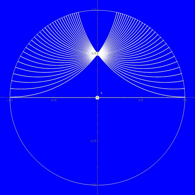
In SU(1,1) straight lines on the disk we considered three one-parameter subgroups of SU(1,1):

(10) $\begin{eqnarray*} X_1&=&\begin{bmatrix}0&i\\-i&0\end{bmatrix},\\ X_2&=&\begin{bmatrix}0&1\\1&0\end{bmatrix},\\ X_3&=&\begin{bmatrix}i&0\\0&-i\end{bmatrix}. \end{eqnarray*}$

(11) $\begin{eqnarray*} A_1(t)&=& \exp(tX_1)=\begin{bmatrix}\cosh(t)&i\sinh(t)\\-i\sinh(t)&\cosh(t)\end{bmatrix},\\ A_2(t)&=& \exp(tX_2)=\begin{bmatrix}\cosh(t)&\sinh(t)\\ \sinh(t)&\cosh(t)\end{bmatrix},\\ A_3(t)&=& \exp(tX_3)=\begin{bmatrix}e^{it}&0\\ 0&e^{-it}\end{bmatrix}. \end{eqnarray*}$

We can now use Eq. (7) in order to see which space-time transformations they implement. Again I calculated it obeying Leibniz and using a machine (see From SU(1,1) to Lorentz).

A replica of the Stepped Reckoner of Leibniz form 1923 (original is in the Hannover Landesbibliothek)

Here are the results of the machine work:

(12) $\begin{equation*}L_1(t)=L(A_1(t))=\begin{bmatrix} 1 & 0 & 0 \\ 0 & \cosh (2 t) & -\sinh (2 t) \\ 0 & -\sinh (2 t) & \cosh (2 t)\end{bmatrix},\end{equation*}$

(13) $\begin{equation*}L_2(t)=L(A_2(t))=\begin{bmatrix} \cosh (2 t) & 0 & \sinh (2 t) \\ 0 & 1 & 0 \\ \sinh (2 t) & 0 & \cosh (2 t) \end{bmatrix},\end{equation*}$

(14) $\begin{equation*}L_3(\phi)=L(A_3(\phi))=\begin{bmatrix} \cos (2 \phi ) & \sin (2 \phi ) & 0 \\ -\sin (2 \phi ) & \cos (2 \phi ) & 0 \\ 0 & 0 & 1 \\ \end{bmatrix},\end{equation*}$

The third family is a simple Euclidean rotation in the $(X,Y)$ plane. That is why I denoted the parameter with the letter $\phi.$ In order to “decode” the first two one-parameter subgroups it is convenient to introduce new variable $v$ and set $2t=\mathrm{arctanh}(v).$ The group property $L(t_1)L(t_2)=L(t_1+t_2)$ is then lost, but the matrices become evidently those of special Lorentz transformations, $L_1(v)$ transforming $Y$ and $T$ , leaving $X$ unchanged, and $L_2(v)$ transforming $(X,T)$ and leaving $Y$ unchanged (though with a different sign of $v$ ). Taking into account the identities

(15) $\begin{eqnarray*} \cosh(\mathrm{arctanh} (v))&=&\frac{1}{\sqrt{1-v^2}},\\ \sinh(\mathrm{arctanh} (v))&=&\frac{v}{\sqrt{1-v^2}} \end{eqnarray*}$

we get

(16) $\begin{equation*}L_1(v)=\begin{bmatrix} 1 & 0 & 0 \\ 0 & \frac{1}{\sqrt{1-v^2}} & -\frac{v}{\sqrt{1-v^2}} \\ 0 & -\frac{v}{\sqrt{1-v^2}} & \frac{1}{\sqrt{1-v^2}}\end{bmatrix},\end{equation*}$

(17) $\begin{equation*}L_2(v)=\begin{bmatrix} \frac{1}{\sqrt{1-v^2}} & 0 & \frac{v}{\sqrt{1-v^2}} \\ 0 & 1 & 0 \\ \frac{v}{\sqrt{1-v^2}} & 0 & \frac{1}{\sqrt{1-v^2}} \end{bmatrix},\end{equation*}$

In the following posts we will use the relativistic Minkowski space distance on the hyperboloid for finding the distance formula on the Poincare disk.

The disk and the hyperbolic model

Posted on 2017/04/102017/04/22 by arkajad

The unit disk in the complex plane, together with geometry defined by invariants of fractional linear SU(1,1) action, known as the Poincaré disk, that is the arena of hyperbolic geometry. But why “hyperbolic”? It is time for us to learn, and to use. In principle the answer is given in Wikipedia, under the subject “Poincaré disk model”. There we find the following picture

with formulas:

Transformation between hyperboloid and disk

We want to derive these formulas ourselves. Let us first introduce our private notation. The hyperboloid will live in a three-dimensional space with coordinates $X,Y,T.$ This is the space-time of Special Relativity Theory, but in a baby version, with $Z$ coordinate suppressed.

The light cone in our space-time has the equation $T^2-X^2-Y^2=0.$ Of course we assume the constant speed of light $c=1.$ Inside the future light cone (the part with $Tgeq 0$ ) there is the hyperboloid defined by $T=\sqrt{1+X^2+Y^2}.$ The coordinates $(X,Y,T)$ of events on this hyperboloid satisfy the equation

(1) $\begin{equation*}T^2-X^2-Y^2=1.\end{equation*}$

As can be seen from the picture above, every straight line passing through the point with coordinates $X_0=Y_0=0,$ $T_0=-1$ and a point with coordinates $(X,Y,T)$ on the hyperboloid, intersects the unit disk at the plane $T=0$ at a point with coordinates $(x,y)$ . We want to find the relation between $(X,Y,T)$ and $(x,y).$

Given any two points, $P=(X_0,Y_0,T_0),$ $Q=(X_1,Y_1,T_1)$ , the points $(X,Y,T)$ on the line joining $P$ and $Q$ have coordinates $(X(u),Y(u),T(u))$ parametrized by a real parameter $u$ as follows:

(2) $\begin{equation*}(X(u),Y(u),T(u))=(1-u)(X_0,Y_0,T_0)+u(X_1,Y_1,T_1).\end{equation*}$

For $u=0$ we are at $P,$ for $u=1$ we are at $Q$ , and for other values of $u$ we are somewhere on the joining line. Our $P$ has coordinates $(0,0,-1),$ our $Q$ has coordinates $(X,Y,T)$ on the hyperboloid, and we are seeking the middle point with coordinate $(x,y,0).$ So we need to solve equations

(3) $\begin{eqnarray*} x&=&(1-u)0+uX=uX,\\ y&=&(1-u)0+uY=uY,\\ 0&=&(1-u)(-1)+uT. \end{eqnarray*}$

From the last equation we find immediately that $u=1/(1+T),$ and the first two equations give us

(4) $\begin{eqnarray*} x&=&\frac{X}{1+T},\\ y&=&\frac{Y}{1+T}. \end{eqnarray*}$

We need to find the inverse transformation. First we notice that

$x^2+y^2=\frac{X^2+Y^2}{(1+T)^2}=\frac{T^2-1}{(1+T)^2}=\frac{T-1}{T+1}.$

Therefore $1-(x^2+y^2)=\frac{2}{T+1}$ and so

$T+1=\frac{2}{1-x^2-y^2},$

$T=\frac{1+x^2+y^2}{1-x^2-y^2}.$

Using Eqs. (4) we now finally get

(5) $\begin{eqnarray*} X&=&\frac{2x}{1-x^2-y^2},\\ Y&=&\frac{2y}{1-x^2-y^2},\\ T&=&\frac{1+x^2+y^2}{1-x^2-y^2}. \end{eqnarray*}$

Thus we have derived the formulas used in Wikipedia. Wikipedia mentions also that the straight lines on the disk, that we were discussing in a couple of recent posts, are projections of sections of the hyperboloid by planes. We will not need this in the future. But we will use the derived formulas for obtaining the relation between SU(1,1) matrices and special Lorentz transformations of space-time events coordinates. This is the job for the devil of the algebra!

Hyperbolic geometry – more parallels

Posted on 2017/04/092017/04/22 by arkajad

Non-Euclidean geometry was invented because not everybody was happy with the fifth postulate of plane Euclid’s geometry. The fifth postulate can be formulated in several equivalent ways, one of its versions, the one that is of interest for us, states that for every straight line and every point that is not on this line, there is a unique parallel line passing through this point. The definition of parallel lines is that they extend infinitely long in both direction without intersection.

Many mathematicians believed that the fifth postulate should somehow follow from other postulates – until models of geometry were constructed with all other postulates satisfied, but the fifth postulate violated. Hyperbolic geometry of the disk that we are studying has this property.

We started playing with parallel lines of the disk geometry in the last post. We will continue it now, but, for change, we will play a little bit more with the devil of the algebra.

Our hyperbolic geometry model is based on invariants of the fractional linear action of SU(1,1) on the unit disk $D$ in the complex plane. The group SU(1,1) acts transitively on the disk. In SU(1,1) decomposition we have seen that every matrix $A$ in SU(1,1) can be uniquely decomposed into a product $A=P(z)U(\theta),$ with $P(z),\, z\in D,$ positive and $U(\theta)$ unitary, both in SU(1,1).

(1) $\begin{equation*} P(z)=\frac{1}{\sqrt{1-|z|^2}}\begin{bmatrix}1&\bar{z}\\ z&1\end{bmatrix},\end{equation*}$

(2) $\begin{equation*}U(\theta)=\begin{bmatrix}e^{i\theta}&0\\0&e^{-i\theta}\end{bmatrix}.\end{equation*}$

The fractional linear transformation defined by $P(z)$ maps the origin $0\in D$ to $z.$

Remark: Given a complex $2\times 2$ matrix $A=\left(\begin{smallmatrix}\lambda&\mu\\ \nu&\rho\end{smallmatrix}\right)$ we define its action on the complex plane by the fractional linear transformation

(3) $\begin{equation*} A:z\mapsto \frac{\rho z+\nu}{\mu z+\lambda}.\end{equation*}$

This is our choice. Another possible choice, that is often used, would be $(\lambda z+\mu)/(\nu z+\rho).$

The matrix $P(z)$ is positive, but positivity is not an intrinsic (or “natural”) property within SU(1,1). If $S$ is in SU(1,1), then the matrix $SP(z)S^{-1}$ is “similar” to $P(z),$ but it is not necessarily positive. While it also has positive eigenvalues, it is not necessarily Hermitian. Intrinsic, natural, properties should be invariant under similarity transformations. Therefore, if only for esthetic reasons, for beauty and for pleasure, we will take now a different road. Within the group SU(1,1) there are special matrices known as parabolic. Parabolic matrices are characterized by the property that they have trace equal 2. This property is invariant under similarity transformations. Our matrix $P(z)$ has trace different from 2. But we can compensate it by multiplying from the right by a unitary matrix, and that is what we will do now.

Multiplying $P(z)$ with $U(\theta)$ from the right we get

(4) $\begin{equation*}P(z)U(\theta)=\frac{1}{\sqrt{1-|z|^2}}\begin{bmatrix}e^{i\theta}&\bar{z}e^{-i\theta}\\ ze^{i\theta}&e^{-i\theta}\end{bmatrix}.\end{equation*}$

If we want to obtain trace equal 2, we should have

(5) $\begin{equation*}\cos \theta=\sqrt{1-|z|^2}.\end{equation*}$

If $\cos \theta=\sqrt{1-|z|^2},$ then for $\sin \theta$ we have two possibilities:

(6) $\begin{equation*}\sin \theta=\pm|z|.\end{equation*}$

Let us choose the first possibility. Then $e^{i\theta}=\sqrt{1-|z|^2}+i|z|,\, e^{-i\theta}=\sqrt{1-|z|^2}-i|z|.$

We define, for each $z$ in the disk, the matrix $Q(z)$ as

(7) $\begin{equation*}Q(z)=P(z)U(\theta)= \begin{bmatrix}1+\frac{i|z|}{\sqrt{1-|z|^2}}&\bar{z}(1-\frac{i|z|}{\sqrt{1-|z|^2}})\\ z(1+\frac{i|z|}{\sqrt{1-|z|^2}})&1-\frac{i|z|}{\sqrt{1-|z|^2}}\end{bmatrix}.\end{equation*}$

With this definition $Q(z)$ maps $0$ to $z$ as before, but now $Q(z)$ is parabolic.

In Hyperbolic geometry – Playing with parallels we were constructing SU(1,1) transformations that were mapping the straight line on the real axis on the disk into parallel lines that were limiting parallel lines – they asymptotically converged to the points $z=-1$ or $z=1$ on the unit circle – the boundary of the disk:

Here I will do the same, but using a different method, with parabolic transformations. The advantage will be that all will be clean algebraic, no hyperbolic or trigonometric functions will be needed. The devil of the algebra will be collaborating with the angel of geometry in one common project.

Let us find $Q(z)$ that leave the point $z=1$ fixed. Using Eqs. (3 and (7) we obtain

(8) $\begin{equation*}1-\frac{i|z|}{\sqrt{1-|z|^2}}+z(1+\frac{i|z|}{\sqrt{1-|z|^2}})=\bar{z}(1-\frac{i|z|}{\sqrt{1-|z|^2}})+1+\frac{i|z|}{\sqrt{1-|z|^2}}.\end{equation*}$

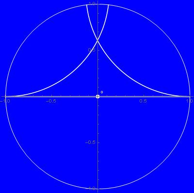
Writing $z=x+iy,$ after some simple manipulations, we obtain a particular solution (I am using Mathematica for such tasks):

$y=\sqrt{x-x^2},$

which makes sense $0\leq x<1.$ Substituting this expression in the formula for $Q(z)$ produces a family $Q_1(x)$ parametrized by $x$

$Q_1(x)=Q(x+i\sqrt{x-x^2})=\begin{bmatrix} \frac{i \sqrt{x}}{\sqrt{1-x}}+1 & \frac{\left(\sqrt{1-x}-i \sqrt{x}\right) \left(x-i \sqrt{-(x-1) x}\right)}{\sqrt{1-x}} \\ \frac{\left(\sqrt{1-x}+i \sqrt{x}\right) \left(x+i \sqrt{-(x-1) x}\right)}{\sqrt{1-x}} & 1-\frac{i \sqrt{x}}{\sqrt{1-x}} \end{bmatrix}.$

The form suggests introducing a new variable, $t=\sqrt{x}/\sqrt{1-x}.$ Then the formula simplifies dramatically:

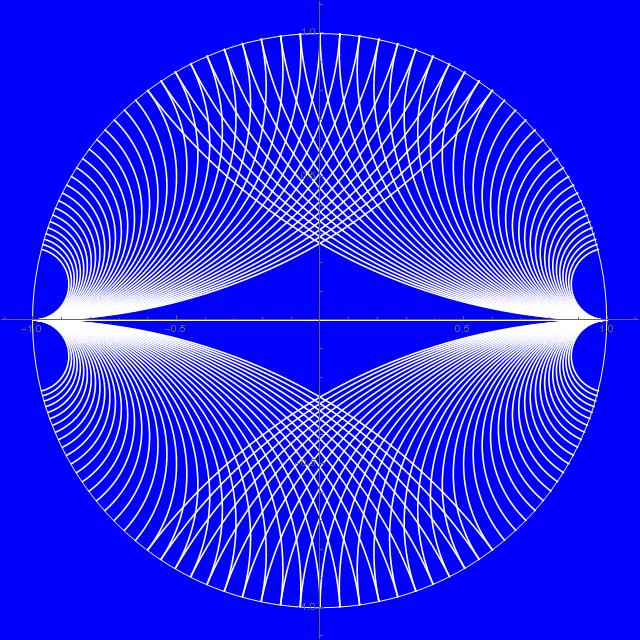
(9) $\begin{equation*}Q_1(t)=\begin{bmatrix} 1+i t & -i t \\ i t & 1-i t \end{bmatrix}.\end{equation*}$

This way we have obtained a very simple family of parabolic transformations, each of them having the point $z=1$ fixed. Below is the result of applying these transformations to the straight line along the real axis for $t=\pm 2^s,$ with $s$ in the range $(-2,2),$ step $0.1.$

Hyperbolic geometry right asymptotic parallels

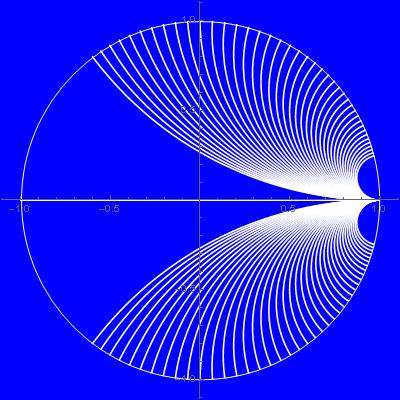
The family $Q_1(t)$ is, in fact, a one-parameter group of parabolic elements in SU(1,1). We have $Q_1(t)Q_1(s)=Q_1(t+s),$ and
$Q_1(t)=\exp tY_1,$ where

(10) $\begin{equation*}Y_1=\begin{bmatrix}i& -i\\i& -i\end{bmatrix}.\end{equation*}$

The matrix $Y_1$ has the “nilpotent” property $Y_1^2=0,$ therefore $\exp tY_1$ reduces to $\exp tY_1=I+tY_1.$

Repeating the same as above, but for $z=-1$ we would get one-parameter group of parabolic matrices $Q_{-1}(t)$

(11) $\begin{equation*}Q_1(t)=\exp t Y_{-1}=\begin{bmatrix} 1-i t & -i t \\ i t & 1+i t\end{bmatrix},\quad Y_{-1}=\begin{bmatrix}-i&-i\\i&i\end{bmatrix}\end{equation*}$

Hyperbolic geometry left and right asymptotic parallels

Let us now return to the transformations $Q_1(t)$ and how they transform the points on the real axis into a segment of a circle – circle according to the Euclidean geometry, straight line according to hyperbolic geometry. Using Eqs. (9) and (3) we get:

(12) $\begin{equation*}Q_1(t):x\mapsto \frac{(1-i t) x+i t}{-i t x+i t+1}=\frac{t^2 (x-1)^2 + x +i(t (x-1)^2)}{1 + t^2 (x-1)^2}.\end{equation*}$

Let us take one particular line, say, for $t=0.4.$ WE easily find that the real part of the expression above vanishes at $x=-1/4.$ the imaginary part at this point is $y=1/2.$ Thus the line defined by $t=0.4$ transformation intersects the vertical imaginary axis at the point $p$ with $y=1/2.$ The same holds for the line defined by $Q_{-1}(0.4).$

We now want to find the formula for all lines parallel to the real axis and crossing the point $p.$ So far we know two of them – the limiting lines:

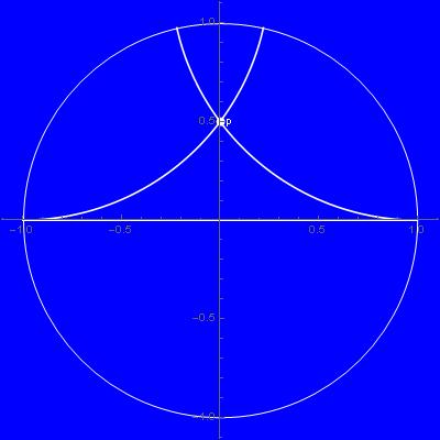
Hyperbolic geometry left and right limiting parallels

First: how to draw all straight lines passing through $p$ ? Simple: we draw straight lines through the origin $z=0,$ which is easy. Then we shift it to the point $p$ using either $P(z_0)$ or $Q(z_0)$ with $z_0=0.5i.$

Here we can see the difference between shifts of straight lines implemented by the parabolic operation $Q(z_0)$ and the positive operation $P(z_0).$

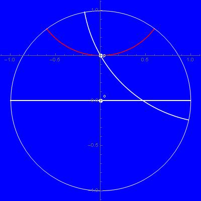
The red line is the shift of real axis by $P(z_0)$ The white line is the shift by $Q(z_0).$ The red line crosses the vertical line, joining $o$ and $p$ , at right angle, in a left-right symmetric way. The white line, on the other hand, crosses the horizontal and the vertical line at the same angle. I did not try to prove it, but it seems from the graph that this is the case. If so, then a proof should be straightforward, and $Q(z)$ could be useful for creating hyperbolic squares and demonstrating that the larger is the square, the smaller is the sum of its four angles.

For our present purpose of creating a family of straight lines through $p$ , and parallel to the real axis, it is more convenient to use $P(z_0)$

(13) $\begin{equation*}P(z_0)=\frac{1}{\sqrt{3}}\begin{bmatrix}2&-i\\i&2\end{bmatrix}.\end{equation*}$

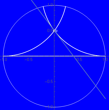
Given angle $\phi,$ $0\leq\phi\leq \pi$ the line through the origin is $re^{i\phi}$ where $r$ varies between $-1$ and 1. We lift it using $P(z_0)$ and get

(14) $\begin{equation*}z(r)=\frac{2re^{i\phi}+i}{-ire^{i\phi}+2}.\end{equation*}$

We look at the left end, for $r=-1,$ and find for which $\phi=\phi_0$ we have $z(-1)=-1.$ That is easy and the result is

(15) $\begin{equation*}\phi_0=\arctan (4/3)=0.927295.\end{equation*}$

In fact, we could obtain this value by examining the angle of intersection of the limiting line with the vertical. I checked it numerically. Geometrical justification is probably easy. Notice that our particular angle happens to be one of the angles of the famous Pythagorean 3-4-5 triangle.