While taking squares is easy, taking square roots may be dangerous. Taking square root of  leads to imaginary numbers. Paul Dirac took square root of the Schrödinger equation, and he has created antimatter. Very dangerous. From Wikipedia:
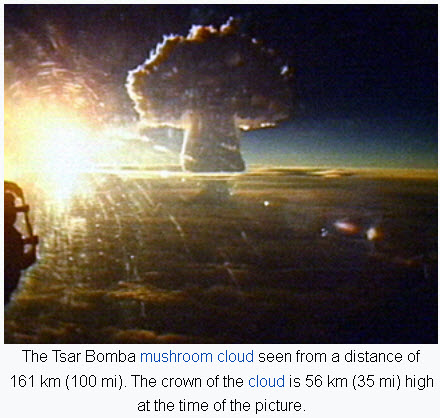
The reaction of 1 kg of antimatter with 1 kg of matter would produce 1.8×10¹⁷ J (180 petajoules) of energy (by the mass–energy equivalence formula, E = mc2), or the rough equivalent of 43 megatons of TNT – slightly less than the yield of the 27,000 kg Tsar Bomb, the largest thermonuclear weapon ever detonated.
Now we want to take square roots of rotations. We will see how dangerous it is. We know that quaternions (equivalently elements of the special unitary group  produce rotations. We even know the exact formula. Given and quaternion
![\[q= W+X\mathbf{i}+Y\mathbf{j}+Z\mathbf{k},\]](http://arkadiusz-jadczyk.eu/blog/wp-content/ql-cache/quicklatex.com-3780159406728af43f0ed4134af0fb82_l3.png "Rendered by QuickLaTeX.com")

(1) 
we have the rotation matrix  given as (see Putting a spin on mistakes):
(2) 
The matrix  is determined by products of the quaternion components. Therefore
  Taking squares is easy. But how to go from
  to
to  ? This amounts to taking square root of the rotation. How do we do it? The problem can be solved, for instance, with a computer algebra system. Here is such a solution:
 define
 (3) 
and
(4) 
Then, with  we have
The following REDUCE code verifies this statement:
OPERATOR R;

MATRIX RR(3,3);

FOR I:=1:3 DO

FOR J:=1:3 DO

RR(I,J):=R(I,J);

R(1,1):=W^2+X^2-Y^2-Z^2;

R(1,2):=2*(X*Y-W*Z);

R(1,3):=2*(W*Y+X*Z);

R(2,1):=2*(W*Z+X*Y);

R(2,2):=W^2-X^2+Y^2-Z^2;

R(2,3):=2*(Y*Z-W*X);

R(3,1):=2*(X*Z-W*Y);

R(3,2):=2*(W*X+Y*Z);

R(3,3):=W^2-X^2-Y^2+Z^2;

LET X**2=1-Y^2-Z^2-W^2;

%LET ABS(W)=W;

s:=2*SQRT(TRACE(RR)+1);

q0:=s/4;

q1:=(R(3,2)-R(2,3))/s;

q2:=(R(1,3)-R(3,1))/s;

q3:=(R(2,1)-R(1,2))/s;

END;
At first sight it looks innocent. We have verified that we have a solution. What else do we need?
Let’s do a test. We take rotations about z-axis (see Mathematics and sex).
![\[\vec{k}=(0,0,1),\]](http://arkadiusz-jadczyk.eu/blog/wp-content/ql-cache/quicklatex.com-7e29156357d371935f6dc45d41ac3ac9_l3.png "Rendered by QuickLaTeX.com")
![\[R_0(t)=\exp tW(\vec{k})=\begin{bmatrix}\cos t&-\sin t&0\\\sin t&\cos t&0\\0&0&1\end{bmatrix}\]](http://arkadiusz-jadczyk.eu/blog/wp-content/ql-cache/quicklatex.com-9b70f8bfb441320acddda1cdbc5752dc_l3.png "Rendered by QuickLaTeX.com")
and tilt by  angle about y axis
  to obtain
(5) 
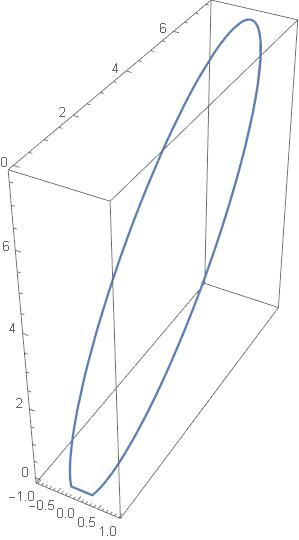
We now use the above map from rotation matrices to quaternions, and then stereographic projection. Mathematica draws the following path:
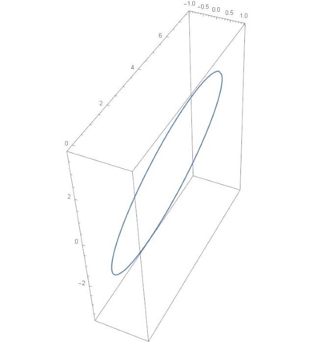
But we know from More recollections that it should look as follows:
Something is evidently going wrong at the bottom pf the plot.
What is going wrong is this: in the formula (3) we divide by  When
When  is very close to
  the calculations become unstable. That is what happens at the bottom of the graph. Mathematica skips the segment for which the precision becomes questionable. Instead of the nice arc, we see a straight line segment there.
In the next post we will be drawing the trajectory of the asymmetric top that is rotating and nutating close to its z axis. In order to avoid instabilities as the one above, we will take special precautions.

 The book
  . A to inna formula


