Before moving to imaginary time let us warm ourselves up first doing a small exercise while still in real time. We did not quite finish our business with periods of elliptic functions in the last post “Periods of Jacobi elliptic functions – Part 1.” We did not answer the question: what about the periods for  ?
?
We know (see The case of inverted modulus – Treading on Tiger’s tail and Jacobi elliptic cn and dn) that for we have the formulas
(1) 
We know, from Periods of Jacobi elliptic functions – Part 1, that the period of  for
for  is
is  Therefore, from Eq. (1) we deduce that the period of for is
  For instance, we have
  But in the previous post we have shown that for we have
(2) 
Therefore, for the period of is  From two last equations in (1) we see that, for , the period for
  is the same as that of , and the period of
  is half of that.
Below is the plot of the function that shows its periodicity.
Plot of for  and
and 
 After these warm-up exercises we now open the door to the universe with the imaginary time. In fact there are several different doors leading there, and we will choose one that has been used by Alfred Cardew Dixon, MA, in his 1894 book “The Elementary Properties of the Elliptic Functions with Examples“.
Namely, we take the Eqs. (1)-(4) from Periods of Jacobi elliptic functions – Part 1 as the defining relations of the Jacobi elliptic functions.
In other words: whenever we have three functions  and a constant
  satisfying
(3) 
(4) 
(5) 
(6) 
(7) 
We are now ready for the trick invented by Jacobi, called “Jacobi Imaginary Transformation“. But before that, once we are in the land of elliptic functions, let us familiarize ourselves with the language used by some of the native population of this country. Following one Dr. Glaisher, the following notation is sometimes used in conversations in local pubs:
![\[\frac{\cn\, u}{\dn\, u}=\mathrm{cd}\, u,\quad \frac{\sn\, u}{\cn\, u}=\mathrm{sc}\, u\]](http://arkadiusz-jadczyk.eu/blog/wp-content/ql-cache/quicklatex.com-828e87da1a618bbcaeb44151fc722e70_l3.png "Rendered by QuickLaTeX.com")
![\[\frac{\dn\, u}{\cn\, u}=\mathrm{dc}\, u,\quad \frac{1}{\sn\, u}=\mathrm{ns}\,u\]](http://arkadiusz-jadczyk.eu/blog/wp-content/ql-cache/quicklatex.com-57ef7822aa3bd2c314d1252ea8186fb2_l3.png "Rendered by QuickLaTeX.com")
![\[\frac{1}{\cn\, u}=\mathrm{nc}\,u,\quad \rm{etc.}\]](http://arkadiusz-jadczyk.eu/blog/wp-content/ql-cache/quicklatex.com-354180f5b8c867625303a43603ed20b7_l3.png "Rendered by QuickLaTeX.com")
Now we are really ready.
It is a question of simple rules about derivatives of fractions and a simple algebra (we can use REDUCE to this end) to establish the following properties:
(8) 
(9) 
(10) 
Here is the REDUCE code checking these relations – it produces, on output, three zeros.:
For all u let sc(u)=sn(u)/cn(u);
For all u let dc(u)=dn(u)/cn(u);
For all u let nc(u)=1/cn(u);
For all u let DF(sn(u),u)=cn(u)*dn(u);
For all v let DF(cn(v),v)=-sn(v)*dn(v);
For all v let DF(dn(v),v)=-k2*sn(v)*cn(v);
For all u let cn(u)^2=1-sn(u)^2;
For all u let dn(u)^2=1-k2*sn(u)^2;
kp2:=1-k2;
l1:=DF(sc(u),u)-dc(u)*nc(u);
l2:=nc(u)^2-sc(u)^2-1;
l3:=dc(u)^2-kp2*sc(u)^2-1;
END;
Comparing Eqs. (8–10) with (3–5) we notice that if we set
![\[S(v)=i\mathrm{sc}\,\,u,\quad C(v)=\mathrm{nc}\, u,\quad D(v)=\mathrm{dc}\, u,\quad v=iu,\quad \lambda=ik'\]](http://arkadiusz-jadczyk.eu/blog/wp-content/ql-cache/quicklatex.com-ec5230e2291ad0f053f7f545da1ec69f_l3.png "Rendered by QuickLaTeX.com")
,
then, since  we must have
  Therefore


 Bu since the relation between
  and
and  is symmetric, we can as well write
(11) 
The functions on the right hand side have the period  denoted simply as
  . Therefore the function on the left hand side have the period
  We can use now addition formula and
calculate the functions  for any complex
  The period along the real direction is
  the period along the imaginary direction is

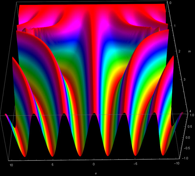
Plot of of the absolute value of  for
for  We have
  ,
, 
Now we can navigate with ease in our complex times. In real time and in imaginary time.