Commenting my statement that “we can now return to the imaginary time period of the pendulum” in my last post Elliptic addition theorem, Bjab aked “What about the real time period?”
And indeed, we did not quite finish the case of the real period. Let me recall what it is about in general terms.
He was seventeen and bored listening to the Mass being celebrated in the cathedral of Pisa. Looking for some object to arrest his attention, the young medical student began to focus on a chandelier high above his head, hanging from a long, thin chain, swinging gently to and fro in the spring breeze. How long does it take for the oscillations to repeat themselves, he wondered, timing them with his pulse. To his astonishment, he found that the lamp took as many pulse beats to complete a swing when hardly moving at all as when the wind made it sway more widely. The name of the perceptive young man, destined to make other momentous scientific discoveries, was Galileo Galilei.
…
Though Galileo discovered the isochronism of the pendulum as a fact of nature, he did not offer an underlying reason for his seminal observation. That explanation had to wait for the great work of Isaac Newton.(From “Galileo’s Pendulum: From the Rhythm of Time to the Making of Matter“, by Roger. G. Newton
Later it was discovered that the isochronism of the pendulum is not the fact of nature. Nevertheless, quoting from “Thus Spoke Galileo: The great scientist’s ideas and their relevance to the present day” by Andrea Frova and Mariapiera Marenzana:
It is interesting to note that Galileo’s mistake in treating this isochronism as perfect led to some important scientific and technological advances. Without this error, for example, perhaps no one would ever have thought of using the pendulum as a device for measuring time.

After this introduction let us do some simple math. In fact, we have already started to discuss the problem in “Nonlinear pendulum period and Kozyrev’s mirrors“. We have noticed that for the mathematical pendulum with the swinging amplitude  smaller than
  we have the formula:
![\[T(m)=\frac{4K(1/m)}{\omega},\]](http://arkadiusz-jadczyk.eu/blog/wp-content/ql-cache/quicklatex.com-4a29bde95839dd3fdcc8d809661a66af_l3.png "Rendered by QuickLaTeX.com")
where  and
and
![\[K(m)=F(\pi/2,m)=\int_0^{\pi/2}\frac{d\theta}{\sqrt{1-m\sin^2\theta}}.\]](http://arkadiusz-jadczyk.eu/blog/wp-content/ql-cache/quicklatex.com-f3f9ff0f98f9652822358e7c75f0b9fd_l3.png "Rendered by QuickLaTeX.com")
The “classical period” from the schoolbooks, one that is a good approximation for small oscillations is
![\[ T_0=\frac{2\pi}{\omega},\]](http://arkadiusz-jadczyk.eu/blog/wp-content/ql-cache/quicklatex.com-79b72c97cabeee1a79df7f344768628d_l3.png "Rendered by QuickLaTeX.com")
where
![\[\omega =\sqrt{\frac{g}{l}.\]](http://arkadiusz-jadczyk.eu/blog/wp-content/ql-cache/quicklatex.com-22edadbd2b7002b46e48ad3b4921c2ff_l3.png "Rendered by QuickLaTeX.com")
In the discussion under that post we have also found the relation between the value of  and the amplitude of the oscillations
![\[\frac{1}{k}=\sin\frac{\alpha}{2}.\]](http://arkadiusz-jadczyk.eu/blog/wp-content/ql-cache/quicklatex.com-49c32a353cd811b9a9a8250d179cca92_l3.png "Rendered by QuickLaTeX.com")
Therefore we can write down the formula telling us how the period of the pendulum depends on the amplitude:
(1) 
where
(2) 
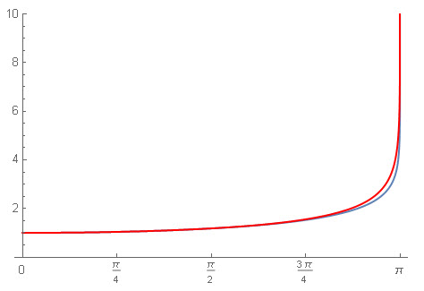
Here is the plot of the function 

We see that it is almost constant and equal to 1 for  . At
. At  we have, in fact:
![\[C(\pi/2)=1.18034,\]](http://arkadiusz-jadczyk.eu/blog/wp-content/ql-cache/quicklatex.com-539322ef070a22b27f761d6450eb90aa_l3.png "Rendered by QuickLaTeX.com")
that is about 18% larger than  . Then the deviation from the constancy of the period becomes larger and larger, and dramatically larger near
  But, of course, experiments with bobs hanging on strings were impossible to conduct for
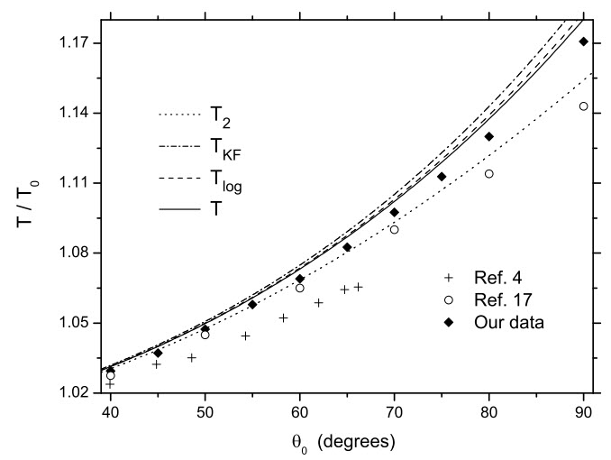
What about experiments with ? How their results fit the theory? What should we tell to students asking such questions? A review can be found in the paper “An accurate formula for the period of a simple pendulum oscillating beyond the small-angle regime” by F. M. S. Lima and P. Arun. They propose a simple approximation to the function  and approximation based on the logarithm function:
![\[C(\alpha)\approx -\frac{\log \cos \frac{\alpha}{2}}{1-\cos\frac{\alpha}{2}}\]](http://arkadiusz-jadczyk.eu/blog/wp-content/ql-cache/quicklatex.com-384e9c2301c58cb838b97729ff8bd3a3_l3.png "Rendered by QuickLaTeX.com")
For comparison I plotted both, where the approximation is in red:
Here is the comparison with experiments, taken from the paper:
Now we are ready to move into imaginary time. In the next post.


Is argument K in (2) OK?
Have you checked if period T (from this post) satisfies formula (1) from former post (Elliptic addition theorem) ?
I have fixed the formulas from this post. Thanks.
They look ok now.
It seems that I need to write more about periods. Tomorrow will do the summary.
Yes, they look OK now.
You changed formula for C(alpha) a lot and got the same plot?
Yes. I was surprised! I do not understand why. A mystery.
That is very strange indeed.
But may be that we have

for
Numerically it seems that there is such an identity
K(m)=K(1/m)/k, m<1
But I can not find it documented somewhere.
It is symmetric, so it does not matter. It looks the same for m as for m’=1/m.
It looks that we have discovered something simple that is not known. I have found a much more complicated formula relating F(x,m) to F{x’,1/m), but not our simple formula.
“It is symmetric, so it does not matter.”
I haven’t noticed that. Thanks.
@Bjab
I have something like a proof of the formula. Wikipedia
has a section about “Differential equation” that is satisfied by K(k).
What I did was: assume that K(k) satisfies this differential equation, and let K1(k)=K(1/k)/k
Then, after long calculation (using computer of course) you find that K1 satisfies the same differential equation.
That is almost a proof (half of it).
You can find a whole chapter (by Milne-Thomson, often cited), a compendium, on elliptic integrals here:
people.math.sfu.ca/~cbm/aands/abramowitz_and_stegun.pdf
And I do not see our simple formula there.
Update: Plots were the same because I was plotting only the real part. There is also imaginary part. It seems that the imaginary part is the second solution of that differential equation, and it gives the imaginary period. But it all needs careful checking. Or finding in some textbook.