Archives for January 2017 | Open System

Crystals of time

Posted on 2017/01/312017/02/23 by arkajad

With title “crystals of time” I am jumping into the future. Indeed, yesterday I received email from one of my colleagues in Russia. He brought to my attention the recent news about “time crystals“: Scientists unveil new form of matter: Time crystals. He has pointed to me that it is something similar to what has been described by Kiwi Bird, and it may have something to do with Dzhanibekov effect that I ma currently in love with. I did not know about the Kiwi Bird, so I checked. Indeed – there is a lot to learn from this bird, and I will have to start studying its songs.

Силуэт птицы киви, соответствующий[1] автору.

Бёрд Ки́ви[2] (также, Киви Берд[3] и kiwibyrd[4]) (от англ. kiwi bird — птица киви) — псевдоним неизвестного автора (группы авторов), который вёл колонку в журнале «Компьютерра», ряде других печатных и онлайновых изданий ИД «Компьютерра» и публикует статьи в журнале «Популярная механика». Основные темы статей — криптография, конспирология и теория заговора.

In short: secret science, conspiracy theories, general scientific weirdness…. A soup made of information mixed with disinformation. Sometimes tastes good.

I looked into the book “Книга о странном”, (Book about Strange) by this strange bird, and of course I have found there the same picture mandala as in my blog post Dzhanibekov effect – Part 2.

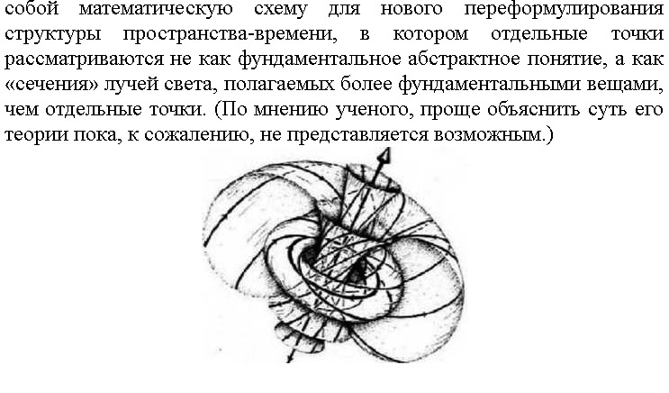
The funny thing is that the book starts with “fractals” – “Глава 1. Фракталы истории” as it is with my post with the picture of the mandala. Strange indeed.

But, as I said, for me all this is in the future. For now I have to continue with Dzhanibekov effect. I am done, more or less, with the mathematics of elliptic functions (I did not even know what elliptic function is a year ago!). We have to return back to physics. In particular I am returning to the content of Dzhanibekov effect – Part 4: The equations of motion.

First recollections (Recollection definition, the act or power of recollecting, or recalling to mind; remembrance).

We consider rigid body. There are no rigid bodies in Nature. That is not a problem for us. Take a stone. It is rigid enough for us, unless someone is crashing it with a hammer. A rigid body has its center of mass. Center of mass of a body does not have to be in the body. Center of mass of an empty cup is somewhere in the air inside the cup. It is a point in space, not necessarily in the body. But somehow the body seems to know where its center of mass is. If there are no external forces or torques acting on the body, as it is, for instance, with a winged nut in Dzhanibekov experiment, then we can well assume that the center of mass is at rest with respect to the inertial frame attached to our laboratory. Classical mechanics tells us then that the angular momentum vector is of constant length and its direction is fixed in space. That is called the law of conservation of the angular momentum.

The fact that physicists call something “a law” does not mean that it is “a true law”. Take for instance a boomerang. It behaves strangely. Physicists explain that boomerang is not really free. There is an air. But what if space is always filled with some kind of “air” or “aether” or “vacuum energy”, and that each body can behave, under certain conditions, like the boomerang, or even stranger, by making use of this “vacuum air”? What if? An I think that it is not just “if”, but that it is really so. There is a lot that waits for being discovered. What then?

Interesting question, but we do not have to deal with this question now. We write it down, in order not to forget, an we simply accept the fact that angular momentum in our situation is conserved with a sufficient approximation to use this “law” in our mathematical idealization of reality. A bird in the hand is worth two in the bush.

What is this angular momentum? It can take a whole book to explain it in all details. But I will take a shortcut.

To a rigid body (a stone, a nut, spinning top) we can attach three mutually orthogonal “principal axes“, a “moving frame“, in such a way that the “inertia tensor” of the body is diagonal, it has three components $I_1,I_2,I_3.$ Here I am recalling the content of Dzhanibekov effect – Part 4: The equations of motion. The relation between components of vectors $\matbf{v}$ in the body frame, and components $\mathbf{V}$ of the same vectors in laboratory frame is given by the “attitude matrix” $Q.$ When the body rotates $Q$ in general depends on time.
…………
That being said I have to pause, and I will continue in the next post. I have to finish reading the book by Olga Kharitidi. I am done with 80% of this book. My impression is that she is mostly inventing her story. It does not sound like a true story. Somewhat similar to Castaneda. Perhaps some kind of “channeling” as well.

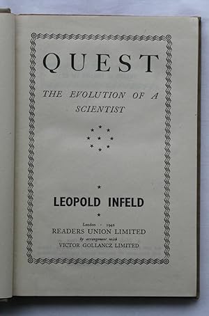
After I am done with Kharitidi, I have waiting for me “Quest: Evolution of a scientist“. This is autobiographical little book by Polish theoretical physicist Leopold Infeld. Infeld was a collaborator of Einstein and his book, published in 1942, has a lot of gossip. To the extent that when another famous Polish physicist, Mathisson, in a discussion with Infeld mentioned that he is reading “Quest”, Infeld asked: “where did you get it?”. Apparently later on Infeld did not want this book to be read. And then, perhaps, I will start reading the Kiwi Bird and time crystals.

Elliptic m-deformed relativity

Posted on 2017/01/302017/02/23 by arkajad

According to Wikipedia special relativity theory was originally proposed in 1905 by Albert Einstein. But Wikipedia is not always the best source of information. For instance Wikipedia has a section about “Causality and prohibition of motion faster than light“. Quite often we can read sentences like that one:

” Since the moving clouds travel slightly slower than the speed of light, they do not actually violate Einstein’s theory of relativity which sets light as the speed limit.”

while elsewhere you can read:

It continues to be alleged that superluminal inﬂuences of any sort would be inconsistent with special relativity for the following three reasons: (i) they would imply the existence of a ‘distinguished’ frame; (ii) they would allow the detection of absolute motion; and (iii) they would violate the relativity of simultaneity. This paper shows that the ﬁrst two objections rest upon very elementary misunderstandings of Minkowski geometry and lingering Newtonian intuitions about instantaneity. The third objection has a basis, but rather than invalidating the notion of faster-than-light inﬂuences it points the way to more general conceptions of simultaneity that could allow for quantum nonlocality in a natural way.

The point is that very often physicists do not think. They repeat what someone told them, or what they read, without much thinking. To quote from “Superluminal motions?A bird-eye view of the experimental situation“, Found.Phys.31:1119-1135,2001, by Erasmo Recami

… Still in pre-relativistic times, one meets various related works, from those by J.J.Thomson to the papers by the great A.Sommerfeld. With Special Relativity, however, since 1905 the conviction spread over that the speed c of light in vacuum was the upper limit of any possible speed. For instance, R.C.Tolman in 1917 believed to have shown by his “paradox” that the existence of particles endowed with speeds larger than c would have allowed sending information into the past. Such a conviction blocked for more than half a century (aside from an isolated paper (1922) by the Italian mathematician G.Somigliana) any research about Superluminal speeds.

Science is not free from “religious wars”. But that is not the subject of my post today. My post is about a certain curious observation that gave me some idea, and I do not know whether this idea is new, or it already occurred to someone else before. And I do not care, because the idea may be not crazy enough to be worth of discussing. Nevertheless it fits the subject of discussion in my recent series, so I will tell it to you now, and, perhaps, ask some questions.

In Special relativity we have a strange formula for addition of velocities (here we will discuss only velocities in one space dimension):

Q & A: Relativistic velocity addition

To simplify the notation I will assume that $c=1,$ or, if you wish, I will understand my velocity $\beta$ as the quotient $u/c$ etc.
The relativistic addition of velocities is sometimes denoted as $u\oplus v$

(1) $\begin{equation*}\beta\oplus \beta'=\frac{\beta+\beta'}{1+\beta\beta'}.\end{equation*}$

John Baez, whom we know from my previous posts, has a web page on How Do You Add Velocities in Special Relativity? There he notices the well know fact that the relativistic addition of velocities is essentially the same as for hyperbolic tangent, where we have

(2) $\begin{equation*}\tanh (x+y)=\frac{\tanh x +\tanh y}{1+\tanh x\tanh y}.\end{equation*}$

One of the consequences of the above addition formula is that if, say $\beta=0.9$ and $\beta'=0.9$ then $\beta\oplus \beta'=0.994475.$
Your spaceship moves with respect to the Sun with velocity that of 90% of the speed of light, and you send from it, in the direction of its flight, a missile traveling with respect to the spaceship with another 90% speed of light, and yet, with respect to the Sun the missile has the speed of 99% of the speed of light, rather than 180% as we would expect from naive addition.

Now, in the recent series of posts we were discussing elliptic functions, and in particular Jacobi sinus function $\sn(u,m).$ We know that for the parameter $m=1$ we have $\sn(u,m)=\tanh u.$ We also have addition formula for $\sn(u,m)$ . It is thus natural to ask how would special relativity look like when the formula (1) is replaced by one derived from the addition formula for $\sn(u,m)$ given in the post Elliptic addition theorem:

(3) $\begin{equation*} \mathrm{sn} (u+v,m)=\frac{\mathrm{sn}(u,m)\mathrm{cn}(v,m)\mathrm{dn}(v,m)+\mathrm{sn}(v,m)\mathrm{cn}(u,m)\mathrm{dn}(u,m)}{1-m\,\mathrm{sn}^2(u,m)\,\mathrm{sn}^2(v,m)}. \end{equation*}$

We can set $\beta=\sn(u,m),\, \beta'=\sn(v,m),$ then $\cn(u,m)=\sqrt{1-\beta^2},\, \dn(u,m)=\sqrt{1-m\beta^2},$ $\cn(v,m)=\sqrt{1-\beta'^2},\, \dn(v,m)=\sqrt{1-m\beta'^2},$ and the new, proposed addition formula, involving parameter $m$ not ncessrily equal to 1, reads:

(4) $\begin{equation*}\beta\oplus_m\beta'=\frac{\beta\sqrt{1-\beta'^2}\sqrt{1-m\beta'^2}+\beta'\sqrt{1-\beta^2}\sqrt{1-m\beta^2}}{1-m\beta^2\beta'^2}. \end{equation*}$

That is my candidate for the m-deformed relativity. How it compares with the non-deformed (that is “standard”) relativity? It looks weird.
Assume our space-ship travels with the speed 90% of the speed of light. Assume $m=0.9$ , and assume we shoot a missile from our ship, in the direction of its motion. What will be the speed of the missile? Here are the plots:

The blue curve is the special relativity. The $0.9\oplus \beta'$ speed always increases, though slower and slower as $\beta'$ approaches 1. But the m-deformed relativity, represented by the red curve is even crazier. If the missile is shot with a speed over a certain value, it starts to move slower with respect to the Sun.

Is that crazy enough to have a chance to be useful?

Can these elliptically deformed addition formulas be included in some geometrical setting? Will it follow from some algebra involving a generalization of the Lorentz group? I do not know.

Moving to imaginary time

Posted on 2017/01/292017/02/23 by arkajad

Before moving to imaginary time let us warm ourselves up first doing a small exercise while still in real time. We did not quite finish our business with periods of elliptic functions in the last post “Periods of Jacobi elliptic functions – Part 1.” We did not answer the question: what about the periods for $m>1$ ?

We know (see The case of inverted modulus – Treading on Tiger’s tail and Jacobi elliptic cn and dn) that for $m>1$ we have the formulas

(1) $\begin{eqnarray*} \sn(u,m)&=&\frac{1}{k}\sn(ku,\frac{1}{m}),\\ \cn(u,m)&=&\dn(ku,1/m),\\ \dn(u,m)&=&\cn(ku,1/m). \end{eqnarray*}$

We know, from Periods of Jacobi elliptic functions – Part 1, that the period of $\sn(u,m)$ for $m<1$ is $4K(m).$ Therefore, from Eq. (1) we deduce that the period of $\sn(u,m)$ for $m>1$ is $4K(1/m)/k.$ For instance, we have $\sn(4K(1/m)/k,m)=\frac{1}{k}\sn(4K(1/m),1/m)=0.$ But in the previous post we have shown that for $m>1$ we have

(2) $\begin{equation*}K(m)=\frac{K(1/m)-iK(1-1/m)}{k}.\end{equation*}$

Therefore, for $m>1$ the period of $\sn(u,m)$ is $4Re(K(m)).$ From two last equations in (1) we see that, for $m>1$ , the period for $\dn(u,m)$ is the same as that of $\sn(u,m)$ , and the period of $\cn(u,m)$ is half of that.
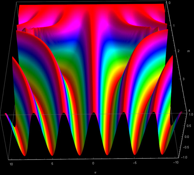
Below is the plot of the function $\dn(u,m)$ that shows its periodicity.

Plot of $\dn(u,m)$ for $|u|<10$ and $0<m<4.$

After these warm-up exercises we now open the door to the universe with the imaginary time. In fact there are several different doors leading there, and we will choose one that has been used by Alfred Cardew Dixon, MA, in his 1894 book “The Elementary Properties of the Elliptic Functions with Examples“.

Namely, we take the Eqs. (1)-(4) from Periods of Jacobi elliptic functions – Part 1 as the defining relations of the Jacobi elliptic functions.
In other words: whenever we have three functions $S(v),C(v),D(v)$ and a constant $\lambda$ satisfying

(3) $\begin{equation*} \frac{d}{dv}\,S= CD,\end{equation*}$

(4) $\begin{equation*} S^2 +C^2=1,\end{equation*}$

(5) $\begin{equation*} D^2+\lambda^2S^2=1,\end{equation*}$

(6) $\begin{equation*}S(0)=0,\quad C(0)=D(0)=1,\end{equation*}$

then

(7) $\begin{equation*}S(v)=\sn(v,\lambda),\,C(v)=\cn(v,\lambda),\,D(v)=\dn(v,\lambda).\end{equation*}$

We are now ready for the trick invented by Jacobi, called “Jacobi Imaginary Transformation“. But before that, once we are in the land of elliptic functions, let us familiarize ourselves with the language used by some of the native population of this country. Following one Dr. Glaisher, the following notation is sometimes used in conversations in local pubs:

$\frac{\cn\, u}{\dn\, u}=\mathrm{cd}\, u,\quad \frac{\sn\, u}{\cn\, u}=\mathrm{sc}\, u$

$\frac{\dn\, u}{\cn\, u}=\mathrm{dc}\, u,\quad \frac{1}{\sn\, u}=\mathrm{ns}\,u$

$\frac{1}{\cn\, u}=\mathrm{nc}\,u,\quad \rm{etc.}$

Now we are really ready.
It is a question of simple rules about derivatives of fractions and a simple algebra (we can use REDUCE to this end) to establish the following properties:

(8) $\begin{equation*} \frac{d}{du} \mathrm{sc}\,u =\mathrm{dc}\,u\,\mathrm{nc}\,u,\end{equation*}$

(9) $\begin{equation*}\mathrm{nc}^2\,u-\mathrm{sc}^2\,u=1,\end{equation*}$

(10) $\begin{equation*}\mathrm{dc}^2\,u-k'^2\mathrm{sc}^2\,u=1, \quad k'=\sqrt{1-k^2}.\end{equation*}$

Here is the REDUCE code checking these relations – it produces, on output, three zeros.:

OPERATOR cn,sn,dn,sc,dc,nc;
For all u let sc(u)=sn(u)/cn(u);
For all u let dc(u)=dn(u)/cn(u);
For all u let nc(u)=1/cn(u);
For all u let DF(sn(u),u)=cn(u)*dn(u);
For all v let DF(cn(v),v)=-sn(v)*dn(v);
For all v let DF(dn(v),v)=-k2*sn(v)*cn(v);
For all u let cn(u)^2=1-sn(u)^2;
For all u let dn(u)^2=1-k2*sn(u)^2;
kp2:=1-k2;
l1:=DF(sc(u),u)-dc(u)*nc(u);
l2:=nc(u)^2-sc(u)^2-1;
l3:=dc(u)^2-kp2*sc(u)^2-1;
END;

Comparing Eqs. (8–10) with (3–5) we notice that if we set

$S(v)=i\mathrm{sc}\,\,u,\quad C(v)=\mathrm{nc}\, u,\quad D(v)=\mathrm{dc}\, u,\quad v=iu,\quad \lambda=ik'$

,
then, since $S(0)=0,C(0)=D(0)=1,$ we must have $S(v)=\sn(v,k'),\,C(v)=\cn(v,k'),\,D(v)=\dn(v,k').$ Therefore
$\sn(iu,k')=i\mathrm{sc}(u,k),$ $\cn(iu,k')=\mathrm{nc}(u,k),$ $\mathrm{dn}(iu,k')=\mathrm{dc}(u,k).$ Bu since the relation between $k$ and $k'$ is symmetric, we can as well write

(11) $\begin{eqnarray*} \sn(iu,k)&=&i\mathrm{sc}(u,k'),\\ \cn(iu,k)&=&\mathrm{nc}(u,k'),\\ \mathrm{dn}(iu,k)&=&\mathrm{dc}(u,k'). \end{eqnarray*}$

The functions on the right hand side have the period $4K(k'),$ denoted simply as $4K'$ . Therefore the function on the left hand side have the period $4iK'.$ We can use now addition formula and
calculate the functions $sn\,z, \cn\,z,\dn\, z$ for any complex $z.$ The period along the real direction is $4K,$ the period along the imaginary direction is $4iK'.$