This is a simple continuation from the last post “Taming the T-handle“. We ended up with the equation
(1) 
where
(2) 
To find  let us assume that
  , we need to integrate
![\[\psi(t)=c_1 t+c_2\int_0^t \frac{1}{1+c_3\,\sn^2(Bs,m)}\,ds.\]](http://arkadiusz-jadczyk.eu/blog/wp-content/ql-cache/quicklatex.com-ea3e6200ed5d48aeecee2d285ceaeff3_l3.png "Rendered by QuickLaTeX.com")
Setting  we transform the above into
![\[\psi(t)=c_1 t+\frac{c_2}{B}\int_0^{Bt} \frac{1}{1+c_3\,\sn^2(u,m)}\,du.\]](http://arkadiusz-jadczyk.eu/blog/wp-content/ql-cache/quicklatex.com-8f00137cbc091f3e923c6ae340ea9705_l3.png "Rendered by QuickLaTeX.com")
Searching the net we can find the integral of this type, for instance on the Wolfram’s page about elliptic integrals of the third order we can find:
![\[\Pi(n;z|m)=\int_0^{F(z|m)}\,\frac{1}{1-n\,\sn(u|m)^2}\, du.\]](http://arkadiusz-jadczyk.eu/blog/wp-content/ql-cache/quicklatex.com-70f1696c4ca67aa612aa0f34df3c4bad_l3.png "Rendered by QuickLaTeX.com")
Then we set  therefore
  – see Jacobi amplitude- realism or cubism,
so that
![\[\psi(t)=c_1 t+\frac{c_2}{B}\,\Pi(-c_3;\am(Bt,m)|m).\]](http://arkadiusz-jadczyk.eu/blog/wp-content/ql-cache/quicklatex.com-4cd54c7375e541d227101a7710b38a10_l3.png "Rendered by QuickLaTeX.com")
In principle we could now substitute the values of  and consider our task essentially done. But that would be not very prudent! The point is that we have the parameter
  and, depending on the case, this parameter can have value:
 and
and  The case
  is very special and should be treated separately. No elliptic functions are needed in this case. Moreover not every software used for calculations and simulations will know what to do with
  and even if it pretends to know, it may happen that in this domain the software is not sufficiently tested and debugged. It is for this reason that we now consider the three cases separately.
The case of  i.e.
i.e. 
This is the most straightforward case. From Taming the T-handle, Eq. (10), we have
(3) 
(4) 
Thus
![\[\frac{c_2}{B}=(I_3-I_1)\sqrt{\frac{I_2}{I_1I_3(I_3-I_2)(1-dI_1)}},\]](http://arkadiusz-jadczyk.eu/blog/wp-content/ql-cache/quicklatex.com-550f7c2e7cc0b40b67d4c4cd712dbb7c_l3.png "Rendered by QuickLaTeX.com")
and we are done.
The case of  i.e.
i.e. 
This is a tricky case. For we have (see Jacobi Elliptic Functions, Eqs. (33)-(35), and this comment)
(5) 
To find  we need to integrate
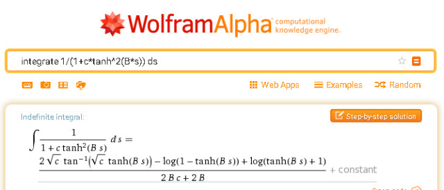
![\[\psi(t)=c_1 t+c_2\int_0^t \frac{1}{1+c_3\,\tanh^2(Bs,m)}\,ds.\]](http://arkadiusz-jadczyk.eu/blog/wp-content/ql-cache/quicklatex.com-790f7cfa0ebf87849fb5a4282521e6e2_l3.png "Rendered by QuickLaTeX.com")
We can go to Wolfram Alpha, and ask it to integrate it. It will, but we will not like the answer. It looks very-very ugly!
In principle we could try to simplify it, but it is better to make one step back in order to make two steps forward! Let us go back to Eq. (1) and write it as just one fraction:
(6) 
 and get
 (7) 
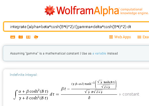
So, we need to integrate the function
(8) 
We can go again to Wolfram Alpha and what we get this time is so much nicer!
All we have to substitute the constants. It is a mechanical task, so we can use REDUCE, so we use REDUCE or any other software capable of symbolic computation. I used Mathematica. Here is the result, followed by a complete summary of the case:
(9) 
(10) 
(11) 
(12) 
(13) 
(14) 
(15) 
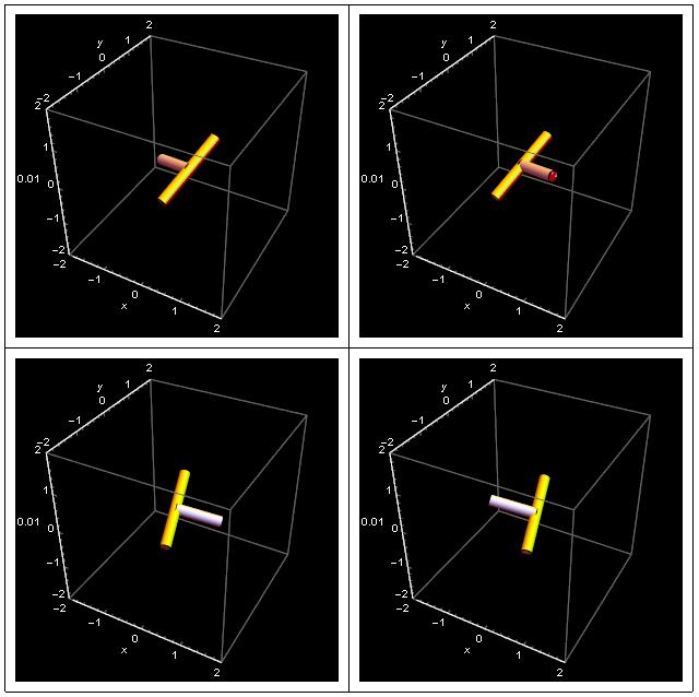
Changing signs of any two of three components  we can obtain altogether four different evolutions of a painted T_handle. But that, and also the case of
  must wait for the next post.
But here are four pictures of the painted T-handle, rotated according to the above algorithm, at  where the three last cases correspond to flipped sign of as follows:
Update
You can download my experimental Mathematica cdf file that can be run using free CDF Player. It shows the code and the animation for the four cases mentioned above.


